VLOOKUP without #N/A error in Excel

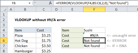
This tutorial shows how to calculate VLOOKUP without #N/A error in Excel using the example below;

Formula

=IFERROR(VLOOKUP(value,table,2,FALSE),"")

Explanation

To hide the #N/A error that VLOOKUP throws when it can’t find a value, you can use the IFERROR function to catch the error and return any value you like.

How the formula works

When VLOOKUP can’t find a value in a lookup table, it returns the #N/A error. The IFERROR function allows you to catch errors and return your own custom value when there is an error. If VLOOKUP returns a value normally, there is no error and the looked up value is returned. If VLOOKUP returns the #N/A error, IFERROR takes over and returns the value you supply.

If you have a lookup value in cell A1 and lookup values in a range named table, and you want a cell to be blank if no lookup is found, you can use:

=IFERROR(VLOOKUP(A1,table,2,FALSE),"")

If you want to return the message “Not found” when no match is found, use:

=IFERROR(VLOOKUP(A1,table,2,FALSE),"Not found")

IFNA option

In Excel 2013, the IFNA function is available to trap and handle #N/A errors specifically. The usage syntax is the same as with IFERROR:

=IFERROR(VLOOKUP(A1,table,2,FALSE),"Not found")
=IFNA(VLOOKUP(A1,table,2,FALSE),"Not found")

Older versions of Excel

In earlier versions of Excel that lack the IFERROR function, you’ll need to repeat the VLOOKUP inside an IF function that catches an error with ISNA or ISERROR. For example:

=IF(ISNA(VLOOKUP(A1,table,2,FALSE)),"",VLOOKUP(A1,table,2,FALSE))