VLOOKUP from another workbook in Excel
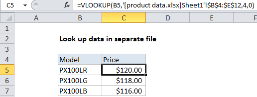
This tutorial shows how to calculate VLOOKUP from another workbook in Excel using the example below;
Formula
=VLOOKUP(B5,[workbook]sheet!range,4,0)

Explanation
To lookup product data, pricing, or other information stored in a separate (external) workbook, you can use the VLOOKUP function with a full reference to the other workbook. In the example shown, the formula in C5 is:
=VLOOKUP(B5,'[product data.xlsx]Sheet1'!$B$5:$E$13,4,0)
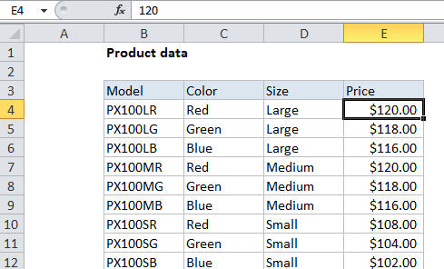
Sample data
The data in the external workbook looks like this:

How this formula works
This is a standard use of the VLOOKUP function to retrieve data from the 4th column in a table:
- lookup value comes from B5
- table_array is a reference to a range in an external workbook
- col_index is 4, to retrieve data from the forth column
- range_lookup is zero to force an exact match
The only difference is the special syntax used for external references, in the “table_array” argument. The syntax for external references is:
'[workbook]sheet'!range
- workbook is the name of the external workbook (i.e. data.xlsx)
- sheet is the name of the sheet containing the range (i.e. Sheet1)
- range is the actual range for table array (i.e. A1:C100)
The easiest way to enter a reference to an external table, is to begin entering the VLOOKUP function normally. Then, when entering the table_array argument, browse to the the external workbook and select the range directly. Excel will construct the needed reference automatically.
Handling spaces and punctuation
Note the reference to workbook is enclosed in square brackets, and the entire workbook + sheet is enclosed in single quotes. The single quotes are required when the workbook or sheet name contains space or punctuation characters