SUMPRODUCT with IF in Excel
This tutorial shows how to SUMPRODUCT with IF in Excel using the example below;
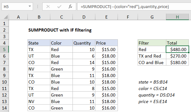
Formula
=SUMPRODUCT(--(color="red"),quantity,price)
Explanation
To filter results of SUMPRODUCT with specific criteria, you can apply simple logical expressions directly to arrays in the function, instead of using the IF function. In the example shown, the formula in H5 is:
=SUMPRODUCT(--(color="red"),quantity,price)
Named ranges
The example uses several named ranges, for convenience only:
state=B5:B14
color=C5:C14
quantity=D5:D14
price=E5:E14
If you’d rather avoid named ranges, use the ranges above entered as absolute references.
How this formula works
This example illustrates one of the key strengths of the SUMPRODUCT function – the ability to filter data with basic logical expressions instead of the IF function. Inside SUMPRODUCT, the first array is a logical expression to filter on the color “red”:
--(color="red")
This results in an array or TRUE FALSE values, which are coerced into ones and zeros with the double negative (–) operation. The result is this array:
{1;0;1;0;0;0;1;0;0;0}
Notice the array contains 10 values, one for each row. A one indicates a row where the color is “red” and a zero indicates a row with any other color.
Next, we have two more arrays: one for quantity and one for price. Together with this results from the first array, we have:
=SUMPRODUCT({1;0;1;0;0;0;1;0;0;0},quantity,price)
Expanding the arrays, we have:
=SUMPRODUCT({1;0;1;0;0;0;1;0;0;0},{10;6;14;9;11;10;8;9;11;10},{15;18;15;16;18;18;15;16;18;16})
SUMPRODUCT’s core behavior is to multiply, then sum arrays. Since we are working with three arrays, we can visualize the operation as shown in the table below, where the result column is the result of multiplying array1 * array2 * array3:
| array1 | array2 | array3 | result |
|---|---|---|---|
| 1 | 10 | 15 | 150 |
| 0 | 6 | 18 | 0 |
| 1 | 14 | 15 | 210 |
| 0 | 9 | 16 | 0 |
| 0 | 11 | 18 | 0 |
| 0 | 10 | 18 | 0 |
| 1 | 8 | 15 | 120 |
| 0 | 9 | 16 | 0 |
| 0 | 11 | 18 | 0 |
| 0 | 10 | 16 | 0 |
Notice array1 works as a filter – zero values here “zero out” values in rows where the color is not “red”. Putting the results back into SUMPRODUCT, we have:
=SUMPRODUCT({150;0;210;0;0;0;120;0;0;0})
Which returns a final result of 480.
Adding additional criteria
You can extend criteria by adding another logical expression. For example, to find total sales where the color is “Red” and the state is “TX”, H6 contains:
=SUMPRODUCT(--(state="tx"),--(color="red"),quantity,price)
Note: SUMPRODUCT is not case-sensitive.
Simplifying with a single array
Excel pros will often simplify the syntax inside SUMPRODUCT a bit by multiplying arrays directly inside array1 like this:
=SUMPRODUCT((state="tx")*(color="red")*quantity*price)
This works because the math operation (multiplication) automatically coerces the TRUE and FALSE values from the first two expressions into ones and zeros.