Summary count by month with COUNTIFS in Excel

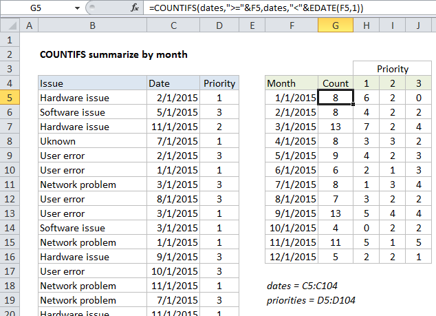
This tutorial shows how to work Summary count by month with COUNTIFS in Excel using the example below;

Formula

=COUNTIFS(dates,">="&A1,dates,"<"&EDATE(A1,1))

Explanation

To create a summary count by month, you can use the COUNTIFS function and the EDATE function with two criteria.

In the example shown, the formula in G5 is:

=COUNTIFS(dates,">="&F5,dates,"<"&EDATE(F5,1))

How this formula works

In this example, we have a list of 100 issues in Columns B to D. Each issue has a date and priority. We are also using the named range “dates” for C5:C104 and “priorities” for D5:D105 .

Starting in column F, we have a summary table that shows a total count per month, and a total count per month per priority.

The first column of the summary table is a date for the first of each month in 2015. Inside COUNTIFS, we need to supply criteria that captures all data by date.  To generate a total count per month, we need criteria that counts all issues that appear in each month.

Since we have actual dates in column F, we can easily construct the criteria we need using the date itself, and a second date created with the EDATE function. These two criteria appear inside COUNTIFS like so:

dates,">="&F5,dates,"<"&EDATE(F5,1)

Roughly translated as “dates greater than or equal to the date in F5 and less than the date in F5 plus one month”.  This is a convenient way to generate “brackets” for each month with one date only.

When the formula is copied down column G, COUNTIFS generates the correct count for each month.

Note: if you don’t want to see full dates in column F, just apply the custom date formats “mmm” or “mmmm” to display the month names only.

With Priority

To generate a count that takes into account priority, we are using this formula in H5:

=COUNTIFS(dates,">="&$F5,dates,"<"&EDATE($F5,1),priorities,H$4)

Here we’ve added an additional criteria range of “priorities” paired with H4 for the criteria itself. In this version of the formula, we get a count by month broken down by the priority, which is picked up directly from row 5.

Notes:

1. The reference to H4 has the row locked (H$4) so priority doesn’t change as the formula is copied down.
2. The reference to F5 has the column locked ($F5) so the date doesn’t change as the formula is copied across.
3. The named ranges “dates” and “priorities” are automatically absolute.