Sum if cells are equal to in Excel

This tutorial shows how to Sum if cells are equal to in Excel using the example below;

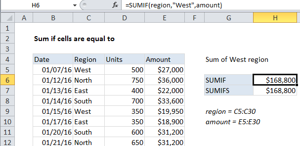
In the example shown, we are summing all sales in the West region.

Explanation

If you need to sum numbers based on other cells being equal to a certain value, you can easily do with either the SUMIF or SUMIFS function.

The formula in cell H6 is:

=SUMIF(region,"West",amount)

The formula in cell H7 is:

=SUMIFS(amount,region,"West")

Both formulas refer to the named ranges region (C5:C30) and amount (E5:E30).

How these formulas work

Both formulas use built-in functions to calculate a subtotal, but the syntax used by SUMIF and SUMIFS is slightly different:

SUMIF(range,criteria,sum_range)
SUMIFS(sum_range,range,criteria)

In both cases, note that the region “West” must be enclosed in double quotes, since it is a text value.

Whether you use SUMIF or SUMIFS (which can handle more than one criteria) is a matter of personal preference. SUMIFS was introduced with Excel 2007, so it’s been around now for a long time.