Sum every nth column in Excel

This tutorial shows how to Sum every nth column in Excel using the example below;

Formula

=SUMPRODUCT(--(MOD(COLUMN(range)-COLUMN(range.first)+1,n)=0),range)

Explanation

To sum every nth column, you can use a formula based on the SUMPRODUCT, MOD, and COLUMN functions.

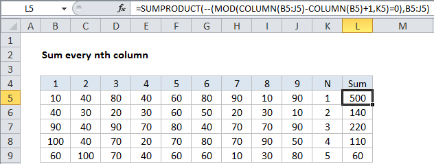
In the example shown, the formula in L5 is:

=SUMPRODUCT(--(MOD(COLUMN(B5:J5)-COLUMN(B5)+1,K5)=0),B5:J5)

How this formula works

At the core, uses SUMPRODUCT to sum values in a row that have been “filtered” using logic based on MOD. The key is this:

MOD(COLUMN(B5:J5)-COLUMN(B5)+1,K5)=0

This snippet of the formula uses the COLUMN function to get a set of “relative” column numbers for the range (explained in detail here) which looks like this:

{1,2,3,4,5,6,7,8,9}

This goes into MOD like so:

MOD({1,2,3,4,5,6,7,8,9},K5)=0

where K5 is the value for N in each row. The MOD function returns the remainder for each column number divided by N. So, for example, when N = 3, MOD will return something like this:

{1,2,0,1,2,0,1,2,0}

Note that the zeros appear for column 3, 6, 9, etc. The formula uses =0 to force a TRUE when the remainder is zero and a FALSE when not, then we use a double-negative (–) to coerce TRUE and FALSE to ones and zeros. That leaves an array like this:

{0,0,1,0,0,1,0,0,1}

Where 1s now indicate “nth values”. This goes into SUMPRODUCT as array1, along with B5:J5 as array2. SUMPRODUCT then does its thing, first multiplying, then summing products of the arrays.

The only values that “survive” multiplication are those where array1 contains 1. In this way, you can think of the logic of array1 “filtering” the values in array2.

Sum every other column

If you want to sum every other column, just adapt this formula as needed, keeping in mind that the formula automatically assigns 1 to the first column in the range. To sum EVEN columns, use:

=SUMPRODUCT(--(MOD(COLUMN(A1:Z1)-COLUMN(A1)+1,2)=0),A1:Z1)

To sum ODD columns, use:

=SUMPRODUCT(--(MOD(COLUMN(A1:Z1)-COLUMN(A1)+1,2)=1),A1:Z1)