Sum columns based on adjacent criteria in Excel

This tutorial shows how to Sum columns based on adjacent criteria in Excel using the example below;

Formula

=SUMPRODUCT(--(range1=criteria),range2)

Explanation

To sum or subtotal columns based on criteria in adjacent columns, you can use a formula based on the SUMPRODUCT function.

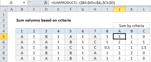
In the example shown, the formula in L5 is:

=SUMPRODUCT(--($B5:$H5=J$4),$C5:$I5)

How this formula works

At the core, uses SUMPRODUCT to multiply then sum products of two arrays: array1 and array2. Array1 is set up to act as a “filter” to allow only values that meet criteria.

Array1 uses a range that begins on the first column that contains values that must pass criteria. These “criteria values” sit in a column to the left of, and immediately adjacent to, the “data values”.

The criteria is applied as a simple test that creates an array of TRUE and FALSE values:

--($B5:$H5=J$4)

This bit of the formula “tests” each value in the first array using the criteria supplied, then uses a double-negative (–) to coerce the resulting TRUE and FALSE values to ones and zeros. The result looks like this:

{1,0,0,0,1,0,1}

Note that 1s correspond to columns 1,5, and 7, which meet the criteria of “A”.

For array2 inside of SUMPRODUCT, we use a range that is “shifted” by one column to the right. This range starts with the first column contain values to sum and ends with the last column that contains values to sum.

So, in the example formula in J5, after the arrays have been populated, we have:

=SUMPRODUCT({1,0,0,0,1,0,1},{1,"B",1,"A",1,"A",1})

Since SUMPRODUCT is programmed specifically to ignore the errors that result from multiplying text values, the final array looks like this:

{1,0,0,0,1,0,1}.