Skip to content
Free Excel Tutorials
  • Home
  • Excel For Beginners
  • Excel Intermediate
  • Advanced Excel For Experts

Data Analysis

  • How To Load Analysis ToolPak in Excel
  • How To Filter Data in Excel
  • Excel Pie Chart
  • Error Bars in Excel
  • Conflicting Multiple Conditional Formatting Rules in Excel

References

  • How to calculate two-way lookup VLOOKUP in Excel Table
  • How to get last row in mixed data with blanks in Excel
  • Offset in Excel
  • Two-column Lookup in Excel
  • How to get last row in text data in Excel

Data Validations

  • Excel Data validation must contain specific text
  • Excel Data validation with conditional list
  • Excel Data validation date in next 30 days
  • Excel Data validation specific characters only
  • Excel Data validation no punctuation

Strikethrough in Excel

by

Apply or remove strikethrough text formatting

This example teaches you how to apply a strikethrough effect to text in Excel. In other words, learn how to draw a line through text in Excel. You can still read text with a strikethrough effect.

1. For example, select the range A2:A4.

2. Right click, and then click Format Cells (or press Ctrl + 1).

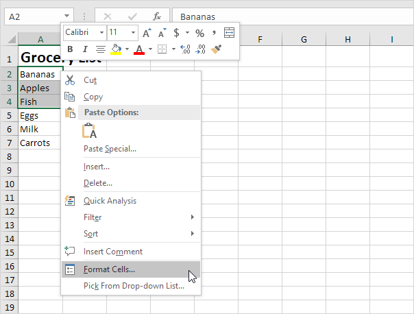
The ‘Format Cells’ dialog box appears.

3. On the Font tab, under Effects, click Strikethrough.
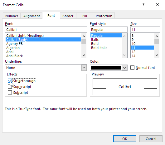
4. Click OK.

Result:

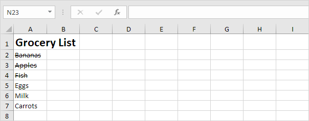
You can also use a keyboard shortcut to quickly apply a strikethrough effect to text in Excel.

5. For example, select cell A7.

6. Press Ctrl + 5.

Result:

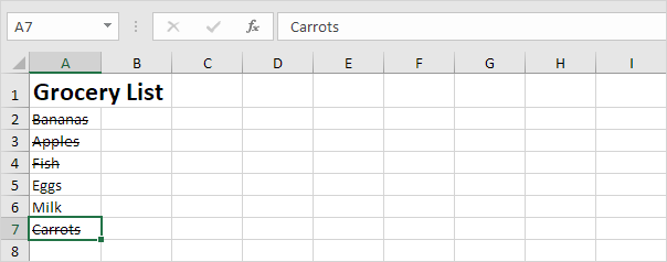
Note: simply press Ctrl + 5 again to remove the strikethrough effect. There’s no double strikethrough option in Excel.

Why cross a text with single or double line in Excel?

Strikethrough resulting in: text like this. Contrary to censored or sanitized (redacted) texts, the words remain readable. This presentation signifies one of two meanings. In ink-written, typewritten, or other non-erasable text, the words are a mistake and not meant for inclusion. When used on a computer screen, however, it indicates recently deleted information, according to wikipedia.

Post navigation

Previous Post:

COSH function: Description, Usage, Syntax, Examples and Explanation

Next Post:

Excel Data validation require unique number

Leave a Reply Cancel reply

Your email address will not be published. Required fields are marked *

Learn Basic Excel

Ribbon
Workbook
Worksheets
Format Cells
Find & Select
Sort & Filter
Templates
Print
Share
Protect
Keyboard Shortcuts

Categories

  • Charts
  • Data Analysis
  • Data Validation
  • Excel Functions
    • Cube Functions
    • Database Functions
    • Date and Time Functions
    • Engineering Functions
    • Financial Functions
    • Information Functions
    • Logical Functions
    • Lookup and Reference Functions
    • Math and Trig Functions
    • Statistical Functions
    • Text Functions
    • Web Functions
  • Excel VBA
  • Excel Video Tutorials
  • Formatting
  • Grouping
  • Others

Logical Functions

  • IF, AND, OR and NOT Functions Examples in Excel
  • How to use IFS function in Excel
  • Nested IF function example in Excel
  • How to return blank in place of #DIV/0! error in Excel
  • IFERROR function: Description, Usage, Syntax, Examples and Explanation

Date Time

  • How to get same date next month or previous month in Excel
  • Add months to date in Excel
  • Convert text date dd/mm/yy to mm/dd/yy in Excel
  • NETWORKDAYS function: Description, Usage, Syntax, Examples and Explanation
  • Display Days in month in Excel

Grouping

  • Map inputs to arbitrary values in Excel
  • Map text to numbers in Excel
  • Group numbers at uneven intervals in Excel
  • Categorize text with keywords in Excel
  • How to randomly assign people to groups in Excel

General

  • AutoFit Column Width, AutoFit Row Height in Excel
  • Freeze and Unfreeze Panes in Excel
  • How to calculate percent sold in Excel
  • How to get original number from percent change in Excel
  • Count cells that contain errors in Excel
© 2026 xlsoffice . All Right Reserved. | Teal Smiles | Abbreviations And Their Meaning