Self-contained VLOOKUP in Excel

To make a self-contained VLOOKUP formula, you can convert the table array to an array constant inside of VLOOKUP.

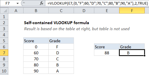
In the example shown the formula in F7 is:

=VLOOKUP(E7,{0,"F";60,"D";70,"C";80,"B";90,"A"},2,TRUE)

How this formula works

Normally, the second argument for VLOOKUP is the table_array, which is input like B6:C10.

When the formula is evaluated, this reference is converted internally to an array like this:

{0,"F";60,"D";70,"C";80,"B";90,"A"}

Note that the comma indicates a column, and semi-colon indicates a row.

Knowing this, when a table is small, you can convert the table to an “array constant” and use the array constant inside VLOOKUP, instead of the reference.

The advantage is that you no longer need the table on the worksheet. The disadvantage is that the array is hard-coded into the formula, and, if you copy the formula to more than one cell, you will have more than one instance of the array to maintain. Editing an array constant is also harder than changing a table on a worksheet.

Named range option

If you want a self-contained table, but don’t want multiple instances of the table in the worksheet, you can create a named range using the array constant, then refer to the the named range in VLOOKUP. The advantage of this approach is that there is only once instance of the table to maintain.