Partial match with VLOOKUP in Excel
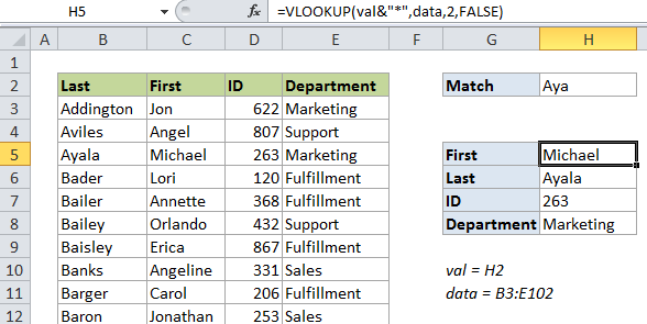
This tutorial shows how to calculate Partial match with VLOOKUP in Excel using the example below;
Formula
=VLOOKUP(value&"*",data,column,FALSE)

Explanation
If you want to retrieve information from a table based on a partial match, you can do so using VLOOKUP in exact match mode, and wildcards.
In the example shown, the VLOOKUP formula looks like this:
=VLOOKUP(val&"*",data,2,FALSE)
In this formula, val is a named range that refers to H2, and data is a named range that refers to B3:E102. Without named ranges, the formula could be written like this:
=VLOOKUP($H$2&"*",$B$3:$E$102,2,FALSE)
How this formula works
VLOOKUP supports wildcards, but only in “exact match” mode. To set exact match, make sure you supply the 4th argument as FALSE or 0.
In this case, we are supplying the lookup value as val&”*”, so if we type in a string like “Aya” into the named range val (H2), we are giving VLOOKUP “Aya*” as the lookup value.
This will cause VLOOKUP to match the first entry in column B that begins with “Aya”.
Wildcard matching is convenient, because you don’t have to type in a full name, but note that you have to be careful of duplicates or near duplicates. For example, in the table there is a “Bailer” and a “Bailey” so typing “Bai” will give you the first match, even though there are two.
Note: it’s important to require an exact match using FALSE or 0 for the last argument when using wildcards.