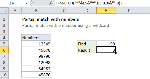
Partial match against numbers with wildcard in Excel
This tutorial shows how to calculate Partial match against numbers with wildcard in Excel using the example below;
Formula
{=MATCH("*"&number&"*",TEXT(range,"0"),0)}

Explanation
To perform a partial match (a substring match) against numbers, you can use an array formula based on MATCH and TEXT.
Background
Excel supports the wildcard characters “*” and “?”. However, if you use wildcards with a number, you’ll convert the numeric value to a text value. In other words, “*”&99&”*” = “*99*” (a text string).
If try to find a text value in a range of numbers, the match will fail.
Solution
One solution is to convert the numbers in the lookup range to text values, and then do a normal lookup with MATCH, VLOOKUP, etc.
If this isn’t practical, you can convert the numeric values to text inside a formula using the TEXT function or by concatenating and empty string to the range.
The formula in E6 is:
{=MATCH("*"&E5&"*",TEXT(B5:B10,"0"),0)}
This is an array formula and must be entered with Control + Shift + Enter
This formula uses the TEXT function to tranform the numbers in B5:B10 to text. Once the numbers are converted to text, the MATCH function can find a partial match as usual.
Note that MATCH must be configured for exact match to use wildcards, by setting the 3rd argument to zero or FALSE.
Another option
Another way to transform a number to text is to concatenate an empty string. This formula works the same as the formula above:
=MATCH("*"&E5&"*",B5:B10&"",0)