Max if criteria match in Excel
This tutorial shows how to calculate Max if criteria match in Excel using the example below;
Formula
{=MAX(IF(criteria_range=criteria,value_range))}

Explanation
To look up the maximum value in a range based on specific critieria, you can use a basic array formula based on the IF function.
Example data and problem
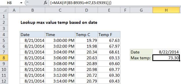
In the example shown, we have almost 10,000 rows of data. The data represents temperature readings taken every 2 minutes over a period of days.
For any given date in the data, we want to get the maximum temperature. We are using cell H7 for the date input.
In the example shown, the formula in cell H8 is:
{=MAX(IF(B5:B9391=H7,E5:E9391))}
Note: this is an array formula and must be entered with Control + Shift + Enter
How this formula works
Inside the IF function, logical test is entered as B5:B9391=H7. Because we’re comparing the value in H7 against a range of cells (an array), the result will be an array of results, where each item in the array is either TRUE or FALSE. The TRUE values represent dates that match H7.
For the value if true, we have E5:E9391, which simply fetches all the values in this range (the temperatures in Fahrenheit). In other words, this also will result in an array of values the same size as the first array.
The IF function returns an array result, which consists of all temperatures where the date matches the value in H7. The IF function only returns items from the 2nd array (temps) where the value in the first array is TRUE.
Finally, the MAX function returns the maximum value from the array delivered by IF.