Skip to content
Free Excel Tutorials
  • Home
  • Excel For Beginners
  • Excel Intermediate
  • Advanced Excel For Experts

Data Analysis

  • How to calculate current stock or inventory in Excel
  • Move chart to a separate worksheet in Excel
  • Conditional Formatting Icon Sets Examples in Excel
  • How to create Checklist in Excel
  • Conditional Formatting New Rule with Formulas in Excel

References

  • Extract data with helper column in Excel
  • Create hyperlink with VLOOKUP in Excel
  • How to get address of named range in Excel
  • Excel Advanced Lookup using Index and Match Functions
  • Lookup entire row in Excel

Data Validations

  • Excel Data validation date in next 30 days
  • Excel Data validation number multiple 100
  • Excel Data validation with conditional list
  • Excel Data validation don’t exceed total
  • Excel Data validation only dates between

Lookup and sum column in Excel

by

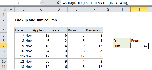
This tutorial shows how to Lookup and sum column in Excel  using the example below;

Formula

=SUM(INDEX(data,0,MATCH(val,header,0)))
Explanation

To lookup and return the sum of a column, you can use the a formula based on the INDEX, MATCH and SUM functions. In the example shown, the formula in I7 is:

=SUM(INDEX(C5:F11,0,MATCH(I6,C4:F4,0)))

How this formula works

The core of this formula uses the INDEX and MATCH function in a special way to return a full column instead of a single value. Working from the inside out, the MATCH function is used to find the correct column number for the fruit in I6:

MATCH(I6,C4:F4,0)

MATCH return 2 inside the INDEX function as the column_num argument, where the array is set to the range C5:F11, which includes data for all fruits.

The tricky part of the formula is the row_num argument, which is set to zero. Setting row to zero causes INDEX to return all values in the matching column in an array like this:

=SUM({6;12;4;10;0;9;6})

The SUM function then returns the sum of all items in the array, 47.

Post navigation

Previous Post:

COSH function: Description, Usage, Syntax, Examples and Explanation

Next Post:

Excel Data validation require unique number

Leave a Reply Cancel reply

Your email address will not be published. Required fields are marked *

Learn Basic Excel

Ribbon
Workbook
Worksheets
Format Cells
Find & Select
Sort & Filter
Templates
Print
Share
Protect
Keyboard Shortcuts

Categories

  • Charts
  • Data Analysis
  • Data Validation
  • Excel Functions
    • Cube Functions
    • Database Functions
    • Date and Time Functions
    • Engineering Functions
    • Financial Functions
    • Information Functions
    • Logical Functions
    • Lookup and Reference Functions
    • Math and Trig Functions
    • Statistical Functions
    • Text Functions
    • Web Functions
  • Excel VBA
  • Excel Video Tutorials
  • Formatting
  • Grouping
  • Others

Logical Functions

  • Invoice status with nested if in Excel
  • XOR function: Description, Usage, Syntax, Examples and Explanation
  • Extract multiple matches into separate rows in Excel
  • Nested IF function example in Excel
  • Excel If, Nested If, And/Or Criteria Examples

Date Time

  • Dynamic date list in Excel
  • Convert Excel time to decimal seconds
  • How to calculate Quarter of Date in Excel
  • Convert date to month and year in Excel
  • Generate series of dates by weekends in Excel

Grouping

  • Group numbers with VLOOKUP in Excel
  • How to randomly assign people to groups in Excel
  • Map text to numbers in Excel
  • Group times into unequal buckets in Excel
  • Running count group by n size in Excel

General

  • Find, Trace and Correct Errors in Excel Formulas using ‘Formula Auditing’
  • How to calculate percent of goal in Excel
  • Currency vs Accounting Format in Excel
  • Excel Operators
  • Transpose: Switch ‘Rows to Columns’ or ‘Columns to Rows’ in Excel
© 2026 xlsoffice . All Right Reserved. | Teal Smiles | Abbreviations And Their Meaning