List sheet names with formula in Excel

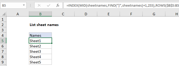
To list worksheets in an Excel workbook, you can use a 2-step approach: (1) define a named range called “sheetnames” with an old macro command and (2) use an INDEX formula to retrieve sheet names using the named range.

Formula

=GET.WORKBOOK(1)&T(NOW())

Note: because this formula relies on a macro command, you’ll need to save as a macro-enabled workbook if you want the formula to continue to update sheet names after the file is closed and re-opened. If you save as a normal worksheet, the sheetname code will be stripped.

Explanation

In the example shown, the formula in B5 is:

=INDEX(MID(sheetnames,FIND("]",sheetnames)+1,255),ROWS($B$5:B5))

How this formula works

The named range “sheetnames” is created with this code:

=GET.WORKBOOK(1)&T(NOW())

GET.WORKBOOK is a macro command that retrieves an array of sheet names in the current workbook. The resulting array looks like this:

{"[workbook.xlsm]Sheet1","[workbook.xlsm]Sheet2","[workbook.xlsm]Sheet3",
"[workbook.xlsm]Sheet4","[workbook.xlsm]Sheet5"}

A cryptic expression is concatenated to the result:

&T(NOW())

The purpose of this code is to force recalculation to pick up changes to sheet names. Because NOW is a volatile function, it recalculates with every worksheet change. The NOW function returns a numeric value representing date and time. The T function returns an empty string (“”) for numeric values, so the concatenation has no effect on values.

Back on the worksheet, cell B6 contains this formula copied down:

=INDEX(MID(sheetnames,FIND("]",sheetnames)+1,255),ROWS($B$5:B5))

Working from the inside out, the MID function is used to remove the worksheet names. The resulting array looks like this:

{"Sheet1","Sheet2","Sheet3","Sheet4","Sheet5"}

This goes into the INDEX function as “array”. The ROW function uses an an expanding ranges to generate an incrementing row number. At each new row, INDEX returns the next array value. When there are no more sheet names to output, the formula will return a #REF error.