if cell contains this or that in Excel

This tutorial shows how to calculate if cell contains this or that in Excel using the example below;

Formula

=IF(SUM(COUNTIF(B5,{"*text1*","*text2*"})),"x","")

Explanation

To check to see if a cell contains more than one substring, you can use a formula based on the COUNTIF function.

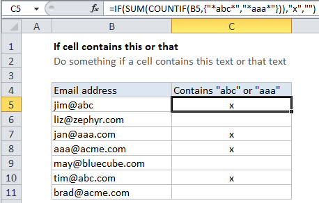
In the example shown, the formula in C5 is:

=IF(SUM(COUNTIF(B5,{"*abc*","*aaa*"})),"x","")

How this formula works

The core of this formula is COUNTIF, which returns zero if none of the substrings is found, and a positive number if at least one substring is found. The twist in this case is that we are giving COUNTIF more than one substring to look for in the criteria, supplied as an “array constant”.  As a result, COUNTIF will return an array of results, with one result per item in the original criteria.

Note that we are also using the asterisk (*) as a wildcard for zero or more characters on either side of the substrings. This is what allows COUNTIF to count the substrings anywhere in the text (i.e. this provides the “contains” behavior).

Because we are getting back an array from COUNTIF, we use the SUM function to sum all items in the array. The result goes into the IF function as the “logical test”.  Any positive number will be evaluated as TRUE, so you can supply any values you like for value if true and value if false.