Skip to content
Free Excel Tutorials
  • Home
  • Excel For Beginners
  • Excel Intermediate
  • Advanced Excel For Experts

Data Analysis

  • How to create dynamic reference table name in Excel
  • How To Load Analysis ToolPak in Excel
  • Chart Axes in Excel
  • Excel Line Chart
  • How to count table columns in Excel

References

  • Last row number in range
  • Get nth match with INDEX / MATCH in Excel
  • Offset in Excel
  • How to get relative column numbers in a range in Excel
  • Lookup entire row in Excel

Data Validations

  • Excel Data validation don’t exceed total
  • Excel Data validation must contain specific text
  • Excel Data validation with conditional list
  • Excel Data validation must not contain
  • How To Create Drop-down List in Excel

How to create dynamic worksheet reference in Excel

by

To create a formula with a dynamic sheet name you can use the INDIRECT function.

Note: The point of this approach is it lets you to build a formula where the sheet name is a dynamic variable. So, for example, you could change a sheet name (perhaps with a drop down menu) and pull in information from different worksheet.

Formula

=INDIRECT(sheet_name&"!A1")

Explanation

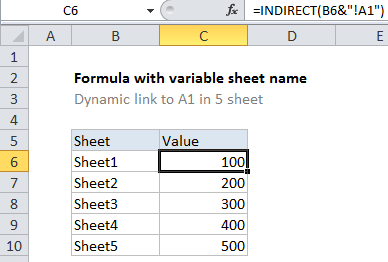
In the example shown, the formula in C6 is:

=INDIRECT(B6&"!A1")

How this formula works

The INDIRECT function tries to evaluate text as a worksheet reference.

In this example, we have Sheet names in column B, so we join the sheet name to the cell reference A1 using concatenation:

=INDIRECT(B6&"!A1")

After concatenation, we have:

=INDIRECT("Sheet1!A1")

INDIRECT recognizes this as a valid reference to cell A1 in Sheet1, and returns the value in A1 (1000).

In cell C7, the formula evaluates like this:

=INDIRECT(B7&"!A1")
=INDIRECT("Sheet2!A1")
=200

And so on, for each formula in column C.

Handling spaces and punctuation in sheet names

If sheet names contain spaces, or punctuation characters, you’ll need to adjust the formula to wrap the sheet name in single quotes like this:

=INDIRECT("'"&sheet_name&"'!A1")

where sheet_name is a cell address like B6 in the example shown.

Post navigation

Previous Post:

DECIMAL function: Description, Usage, Syntax, Examples and Explanation

Next Post:

AVERAGE function: Description, Usage, Syntax, Examples and Explanation

Leave a Reply Cancel reply

Your email address will not be published. Required fields are marked *

Learn Basic Excel

Ribbon
Workbook
Worksheets
Format Cells
Find & Select
Sort & Filter
Templates
Print
Share
Protect
Keyboard Shortcuts

Categories

  • Charts
  • Data Analysis
  • Data Validation
  • Excel Functions
    • Cube Functions
    • Database Functions
    • Date and Time Functions
    • Engineering Functions
    • Financial Functions
    • Information Functions
    • Logical Functions
    • Lookup and Reference Functions
    • Math and Trig Functions
    • Statistical Functions
    • Text Functions
    • Web Functions
  • Excel VBA
  • Excel Video Tutorials
  • Formatting
  • Grouping
  • Others

Logical Functions

  • Nested IF function example in Excel
  • Not Equal To ‘<>‘ operator in Excel
  • AND function: Description, Usage, Syntax, Examples and Explanation
  • IF with boolean logic in Excel
  • How to use Excel NOT Function

Date Time

  • Calculate total hours that fall between two times in Excel
  • Get last weekday in month in Excel
  • Display Date is workday in Excel
  • Convert Excel time to Unix time in Excel
  • Add months to date in Excel

Grouping

  • Map text to numbers in Excel
  • Categorize text with keywords in Excel
  • How to randomly assign data to groups in Excel
  • Calculate conditional mode with criteria in Excel
  • Group numbers with VLOOKUP in Excel

General

  • How to increase by percentage in Excel
  • Excel Ribbon Quick Overview For Beginners
  • Check if multiple cells have same value with case sensitive in Excel
  • How to calculate percent of goal in Excel
  • How to calculate percent of students absent in Excel
© 2026 xlsoffice . All Right Reserved. | Teal Smiles | Abbreviations And Their Meaning