How to create dynamic named range with INDEX in Excel

This page shows an example of a dynamic named range created with the INDEX function together with the COUNTA function. Dynamic named ranges automatically expand and contract when data is added or removed.

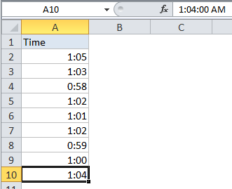
In the example shown, the named range “data” is defined by the following formula:

=$A$2:INDEX($A:$A,COUNTA($A:$A))

which resolves to the range $A$2:$A$10.

How this formulas works

Note first that this formula is composed in two parts that sit either side of the range operator (:). On the left, we have the starting reference for the range, hard-coded as:

$A$2

On the right is the ending reference for the range, created with INDEX like this:

INDEX($A:$A,COUNTA($A:$A))

Here, we feed INDEX all of column A for the array, then use COUNTA to figure out the “last row” in the range. COUNTA works well here because there are 10 values in column A, including a header row. COUNTA therefore returns 10, which goes directly into INDEX as the row number. INDEX then returns a reference to $A$10, the last used row in the range:

INDEX($A:$A,10) // resolves to $A$10

So, the final result of the formula is this range:

$A$2:$A$10

A two dimensional range

The above example works for a one-dimensional range. To create a two-dimensional dynamic range where the number of columns is also dynamic, you can use the same approach, expanded like this:

=$A$2:INDEX($1:$1048576,COUNTA($A:$A),COUNTA($1:$1))

As before, COUNTA is used to figure out the “lastrow”, and we use COUNTA again to get the “lastcolumn”. These are supplied to index as row_num and column_num respectively.

However, for the array, we supply the full worksheet, entered as all 1048576 rows, which allows INDEX to return a reference in a 2D space.

Note: Excel 2003 supports only 65535 rows.