Get nth match with VLOOKUP in Excel
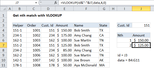
This tutorial shows how to Get nth match with VLOOKUP in Excel using the example below;
Formula
=VLOOKUP(id_formula,table,4,0)
 Explanation
To get the nth MATCH with VLOOKUP, you’ll need to add a helper column to your table that constructs a unique id that includes the count. If this isn’t practical, you can use an array formula based on INDEX and MATCH instead.
=VLOOKUP(id&"-"&I6,data,4,0)
How this formula works
This formula depends on a helper column, which is added as the first column to the source data table. The helper column contains a formula which builds a unique lookup value from an existing id and a counter. The counter counts the number of times the unique id has appeared in the data table.
In the example, the formula cell B4 of the helper column looks like this:
=D4&"-"&COUNTIF($D$4:D4,D4)
This formula picks up the value in D4 and uses concatenation to add a hyphen, and the result of a COUNTIF function. The COUNTIF function uses an expanding range (the mixed reference $D$4:D4) to generate a running count of the id in the data.
On the lookup side, VLOOKUP is used to fetch values form the table, taking into account the “nth” occurrence. The trick is to build a lookup value with the same structure as the values that appear in the helper column, taking into account “nth”. Again, this is done with concatenation, by adding a hyphen and a value that represents “nth” to a normal lookup value (pulled from the named range “id” in this case).