Get first text value with HLOOKUP in Excel

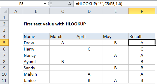
To lookup and retrieve the first text value across a range of columns, you can use the HLOOKUP function with a wildcard. In the example shown, the formula in F5 is:

=HLOOKUP("*",C5:E5,1,0)

How this formula works

Sometimes, you may want to check a range of several columns and extract the first text value found. You can do this with the HLOOKUP function and the asterisk wildcard character (*).

In the formula shown, HLOOKUP is configured like this:

=HLOOKUP("*",C5:E5,1,0)

The lookup value is “*”, a wildcard that matches one or more text values.

The table array C5:E5, entered as a relative references so that it changes as the formula is copied down column F.

The row index number is 1, since the range contains only one row.

The range lookup argument is set to zero (false) to force exact match. This is required when using wildcards with VLOOKUP or HLOOKUP.

In each row, HLOOKUP finds and returns the first text value found in columns C through E in each row.

Ignoring empty strings

To ignore empty strings generated by other formulas, try adjusting wildcards as follows:

=HLOOKUP("?*",range,1,0)

Translated: match text with at least one character.

Note: this formula won’t work for numeric values since the asterisk wildcard matches only text.