Dynamic lookup table with INDIRECT in Excel
This tutorial shows how to calculate Dynamic lookup table with INDIRECT in Excel using the example below;
To allow a dynamic lookup table, you can use the INDIRECT function with named ranges inside of VLOOKUP.
Formula
=VLOOKUP(A1,INDIRECT("text"),column)

Explanation
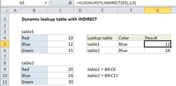
In the example shown the formula in G5 is:
=VLOOKUP(F5,INDIRECT(E5),2,0)
Background
The purpose of this formula is to allow an easy way to switch table ranges inside a lookup function. One way to handle is to create a named range for each table needed, then refer to the named range inside of VLOOKUP. However, if you just try to give VLOOKUP a table array in the form of text (i.e. “table1”) the formula will fail. The INDIRECT function is needed to resolve the text to a valid reference.
How this formula works
At the core, this is a standard VLOOKUP formula. The only difference is the use of INDIRECT to return a valid table array.
In the example shown, two named ranges have been created: “table1” refers to B4:C6, and “table2” refers to B9:C11*.
INDIRECT picks up the text in E5 (“table1”) and resolves it the named range table1, which resolves to B9:C11, which is returned to VLOOKUP.
VLOOKUP performs the lookup and returns 12 for the color “blue” in table1.
* Note: names ranges actually create absolute references like $B$9:$C$11, but I’ve omitted the absolute reference syntax to make the description easier to read.