Count multiple criteria with NOT logic in Excel

This tutorial shows how to Count multiple criteria with NOT logic in Excel using the example below;

Formula

=SUMPRODUCT((range1=criteria1)*ISNA(MATCH(range2,criteria2,0)))

Explanation

To count with multiple criteria, including logic for NOT one of several things, you can use the SUMPRODUCT function together with the MATCH and ISNA functions.

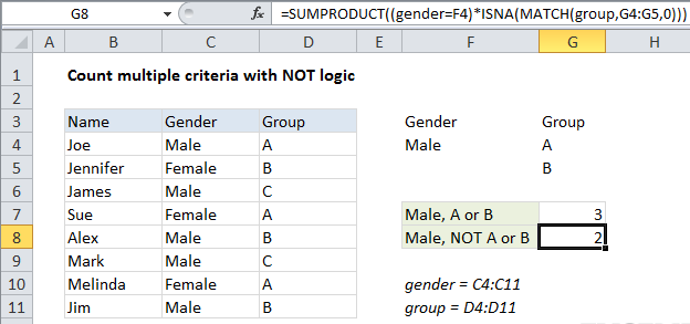
In the example shown, the formula in G8 is:

=SUMPRODUCT((gender=F4)*ISNA(MATCH(group,G4:G5,0)))

Where “gender” is the named range C4:C12, and “group” is the named range D4:D12.

Note: MATCH and ISNA allow the formula to scale easily to handle more exclusions, since you can easily expand the range to include additional “NOT” values.

How this formula works

The first expression inside of SUMPRODUCTS tests values in column C, Gender, against the value in F4, “Male”:

(gender=F4)

The result is an array of TRUE FALSE values like this:

{TRUE;FALSE;TRUE;FALSE;TRUE;TRUE;FALSE;TRUE;FALSE}

Where TRUE corresponds to “Male”.

The second expression inside of SUMPRODUCTS tests values in column D, Group, against the values in G4:G5, “A” and “B”. This test is handled with MATCH and ISNA like this:

ISNA(MATCH(group,G4:G5,0))

The MATCH function is used to match every value in the named range “group” against values in G4:G5, “A” and “B”. Where the match succeeds, MATCH returns a number. Where the MATCH fails, MATCH returns #N/A. The result is an array like this:

{1;2;#N/A;1;2;#N/A;1;2;#N/A}

Since #N/A values correspond to “not A or B”, ISNA is used to “reverse” the array to:

{FALSE;FALSE;TRUE;FALSE;FALSE;TRUE;FALSE;FALSE;TRUE}

Now TRUE corresponds to “not A or B”.

Inside SUMPRODUCT, the two array results are multiplied together, which creates a single numeric array inside SUMPRODUCT:

SUMPRODUCT({0;0;1;0;0;1;0;0;0})

SUMPRODUCT then returns the sum, 2, representing “2 males not in group A or B”.