Count long numbers without COUNTIF in Excel
This tutorial shows how to Count long numbers without COUNTIF in Excel using the example below;
Formula
=SUMPRODUCT(--(A:A=A1))

Explanation
This is an annoyingly long introduction, but the context is important, sorry!
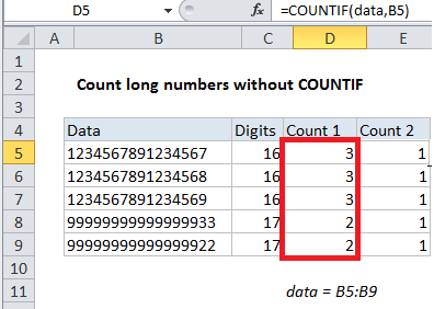
If you try to count very long numbers (16+ digits) in a range with COUNTIF, you may see incorrect results, due to a bug in how certain functions handle long numbers, even when those numbers are stored as text. Consider the screen below. All counts in column D are incorrect —although each number in column B is unique, the count returned by COUNTIF suggests these numbers are duplicates.

Note: All counts are incorrect. Numbers are unique but appears to be duplicated.
=COUNTIF(data,B5)
This problem is related to how Excel handles numbers. Excel can only handle 15 significant digits, and if you enter a number with more than 15 digits in Excel, you’ll see the trailing digits silently converted to zero. The counting problem mentioned above arises from this limit.
Normally, you can avoid this limit by entering long numbers as text, either by starting the number with a single quote (‘999999999999999999) or by formatting the cell(s) as Text before entering. As long as you don’t need to perform math operations on a number, this is a good solution, and it lets you enter extra long numbers for things like like credit card numbers and serial numbers without losing any numbers.
However, if you try to use COUNTIF to count a number with more than 15 digits (even when stored as text) you may see unreliable results. This happens because COUNTIF internally converts the long value back to a number at some point during processing, triggering the 15 digit limit described above. Without all digits present, some numbers may be counted like duplicates when counted with COUNTIF.
Solution
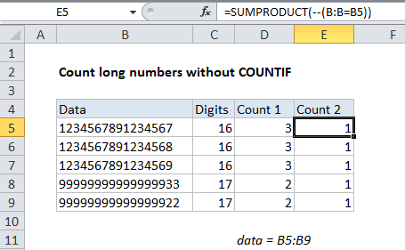
One solution is to replace the COUNTIF formula with a formula that uses SUM or SUMPRODUCT. In the example shown, the formula in E5 looks like this:
=SUMPRODUCT(--(data=B5))
The formula uses the named range “data” (B5:B9) and generates the correct count for each number with SUMPRODUCT.
How this formula works
First, the expression inside SUMPRODUCT compares all values in the named range “data” with the value from column B in the current row. This results in an array of TRUE/FALSE results.
=SUMPRODUCT(--(data=B5))
=SUMPRODUCT(--({TRUE;FALSE;FALSE;FALSE;FALSE}))
Next, the double negative coerces the TRUE/FALSE values to 1/0 values.
=SUMPRODUCT({1;0;0;0;0})
Finally, SUMPRODUCT simply sums the items in the array and returns the result.
Array formula variant
You can also use the SUM function instead of SUMPRODUCT, but this is an array formula and must be entered with control + shift + enter:
{=SUM(--(B:B=B5))}