Count cells that contain errors in Excel

This tutorial shows how to Count cells that contain errors in Excel using the example below;

Formula

=SUMPRODUCT(–ISERR(range))

Explanation

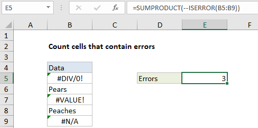
To count cells that contain errors, you can use the ISERR function, wrapped in the SUMPRODUCT function.  In the example shown, E5 cell contains this formula:

=SUMPRODUCT(--ISERROR(B5:B9))

How this formula works

SUMPRODUCT accepts one or more arrays, multiplies the arrays together, and returns the “sum of products” as a final result. If only one array is supplied, SUMPRODUCT simply returns the sum of items in the array.

The ISERROR function returns TRUE when a cell contains an error, and FALSE if not. In the example, ISERROR receives a range of cells (B5:B9) as input. Because there are five cells in the range, ISERROR evaluates each cell and returns five results in an array of TRUE / FALSE values:

{TRUE;FALSE;TRUE;FALSE;FALSE}

To coerce the TRUE/FALSE values to 1’s and 0’s, we use a double negative (called a double unary). The resulting array looks like this:

{1;0;1;0;0}

Finally, SUMPRODUCT sums the items in this array and returns the total, which is 3 in this case.

Note: ISERROR counts all errors. If for some reason you want to count all errors except #N/A, you can use the ISERR function instead.

Array formula with SUM

You can also use the SUM function to count errors, but you must enter as an array formula using control + shift + enter. Once entered the formula will look like this:

{=SUM(--ISERROR(range))}

The curly brackets are added automatically by Excel and indicate an array formula.