Count cells equal to case sensitive in Excel

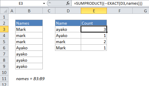
This tutorial shows how to Count cells equal to case sensitive in Excel using the example below;

Formula

=SUMPRODUCT((–EXACT(value,range)))

Explanation

To count cells that contain certain text in a case-sensitive manner, you can use a formula that uses the EXACT function along with SUMPRODUCT.

In the example, there is a list of names in a named range (“names”), B3:B9. In the range D3:D6, there is a another list of names, with duplicates removed. To get the count of “ayako”, you can use the formula:

=SUMPRODUCT((--EXACT("ayako",B3:B9)))

In the example, which uses the named range “names”, the first formula is:

=SUMPRODUCT((--EXACT(D3,names)))

Both formulas above return 3, since there are 3 occurrences of “ayako” (lowercase) in the range B3:B9.

How this formula works

The EXACT function takes to arguments, text1 and text2. When these values match exactly (respecting case), EXACT returns TRUE. In this case, we are giving EXACT a range for text1, so it becomes an array formula and returns an array of TRUE and FALSE values like this:

{FALSE;FALSE;FALSE;FALSE;TRUE;TRUE;TRUE}

Each TRUE represents an exact match of “ayako” in B3:B9.

The double-hypen (technically: double unary) converts the TRUE false values into 1’s and 0’s that look like this:

{0;0;0;0;1;1;1}

Finally, SUMPRODUCT simply adds up the values in the array and returns 3. Because SUMPRODUCT can handle arrays natively, it’s not necessary to use Control+Shift+Enter to enter this formula.