Case sensitive match in Excel
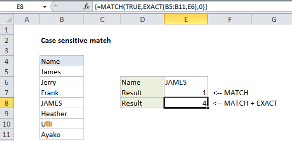
This tutorial shows how to calculate Case sensitive match in Excel using the example below;
Formula
{=MATCH(TRUE,EXACT(range,value),0)}

Explanation
To perform a case sensitive match, you can use the EXACT function together with MATCH in an array formula. In the example show, the formula in E8 is:
{=MATCH(TRUE,EXACT(B5:B11,E6),0)}
Note: this is an array formula and must be entered with Control + Shift + Enter.
How this formula works
By itself, the MATCH function is not case-sensitive, so the following formula returns 1:
=MATCH("JAMES",B5:B11,0)
To add case-sensitivity, we use the EXACT function like this:
EXACT(B5:B11,E6)
Which returns an array of TRUE/FALSE values:
{FALSE;FALSE;FALSE;TRUE;FALSE;FALSE;FALSE}
This array goes into the MATCH function as the lookup_array. For lookup_value, we use TRUE with MATCH set to exact match mode by setting match_type to zero.
=MATCH(TRUE,{FALSE;FALSE;FALSE;TRUE;FALSE;FALSE;FALSE},0)
Match then returns the position of the first TRUE value found: 4.