Calculate grades with VLOOKUP in Excel

If you want to calculate grades using the VLOOKUP function, it’s easy to do. You just need to set up a small table that acts as the “key”, with scores on the left, and grades on the right.

This table must be sorted in ascending order, and VLOOKUP must be configured to do an “approximate match”.

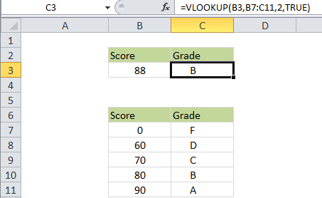
In the example shown, the VLOOKUP formula looks like this:

=VLOOKUP(B3,B7:C11,2,TRUE)

How this formula works

In this case B3 is the score to convert to a grade (88 in the example) B7:C11 is the “grade key”, composed of a 2-column table, 2 tells VLOOKUP to get data from the 2nd column (the grades), and TRUE tells VLOOKUP to do an “approximate match”.

In “approximate match mode” VLOOKUP assumes the table is sorted by the first column. When VLOOKUP finds a value that’s greater than the lookup value, it will fall back, and return a value from the previous row.

In other words, VLOOKUP matches the last value that is less than or equal to the lookup value.

If the first value in the table is less than the value being looked up, VLOOKUP will return the #N/A error.

Note: by default, VLOOKUP will perform an approximate match, so there is no need to supply the 4th argument, since the default is TRUE. However, we recommend you get in the habit of supplying the last argument so that you have a visual reminder of the current match mode.