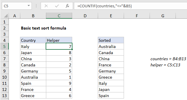
Basic text sort formula in Excel

To dynamically sort text values in alphabetical order, you can use use a formula based on the COUNTIF function.

Formula

=COUNTIF(range,"<="&A1)

Explanation

In the example shown, the formula in C5 is:

=COUNTIF(countries,"<="&B5)

where “countries” is the named range B4:B13

How this formula works

This formula uses the “greater than or equal to” operator with text, something you might not have tried before. When Excel compares text, it decides which value is “greater” than another based rules that follow the ASCII numbering scheme.

Inside COUNTIF, the range argument is supplied as the named range “countries” (B4:B13), and criteria is supplied as “less than or equal to” the value in C5. In each row, COUNTIFS returns the number of values that are less than or equal to the current value, which creates a sequential list of numbers (i.e. a rank) in the helper column.

Handling duplicates

If the data contains duplicate text values, the sequence of sort numbers will also contain duplicates, which will cause problems if you are trying to retrieve values with the INDEX function. To work around this problem, you can use a variation of the formula that increments duplicates with a second COUNTIF:

=COUNTIF(countries,"<"&B5)+COUNTIF($B$5:B5,B5)

Note the logical operator in the first COUNTIF function has been adjusted, and the range in the second COUNTIF function is an expanding reference.

Listing sorted values

The helper column can be used used to retrieve sorted values by rank. In E5, the formula used to retrieve values is:

=INDEX(countries,MATCH(ROWS($E$5:E5),helper,0))

This is an INDEX and MATCH formula that uses an expanding reference to generate sequential numbers, which are fed into MATCH as lookup values. MATCH figures out where each number exists in the data, and INDEX retrieves the value at that position. See this page for a more detailed explanation.