Average response time per month in Excel
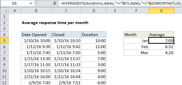
This tutorial shows how to work Average response time per month in Excel using the example below;
Formula
=AVERAGEIFS(durations,dates,">="&A1,dates,"<="&EOMONTH(A1))
Explanation
To average response times by month, you can use a formula based on the AVERAGEIFS function, together with the EOMONTH function.
In the example shown, the formula in G5 is:
=AVERAGEIFS(durations,dates,">="&F5,dates,"<="&EOMONTH(F5,0))
How this formula works
This formula uses the named ranges “dates” (B5:B25) and “durations” (D5:D25). Durations column D are in minutes, calculated by subtracting the date opened from date closed.
The AVERAGEIFS function is designed to average ranges based on multiple criteria. In this case, we configure AVERAGEIFS to average durations by month using two criteria: (1) matching dates greater than or equal to the first day of the month, (2) matching dates less than or equal to the last day of the month.
To bracket dates by month, we use a simple trick to make things easier: In column F, instead of typing month names (“Jan”, “Feb”, Mar”, etc.) we add we add actual dates for the first of each month (1/1/2016, 2/1/2016, 3/1/2016, etc.),. Then, we use the custom date format (“mmm”) to display the month names.
This makes it a lot easier to build the criteria we need for AVERAGEIFS using values in column F. To match dates greater than or equal to the first of the month, we use:
">="&F5
To match dates less than or equal to the last day of the month, we use:
"<="&EOMONTH(F5,0)
We get the EOMONTH to return the last day of the same month by supplying zero for the monthsargument.
Note: concatenation with an ampersand (&) is necessary when building criteria based on a cell reference.
