Average last 5 values in Excel

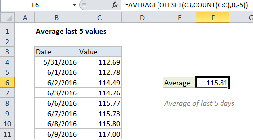
This tutorial shows how to work Average last 5 values in Excel using the example below;

Formula

=AVERAGE(OFFSET(A1,COUNT(A:A),0,-N))

Explanation

To average the last 5 data points, you can use the AVERAGE function together with the COUNT and OFFSET functions. You can use this approach to average the last N data points: last 3 days, last 6 measurements, etc.

In the example shown, the formula in F6 is:

=AVERAGE(OFFSET(C3,COUNT(C:C),0,-5))

How this formula works

The OFFSET function can be used to construct dynamic rectangular ranges. Given a starting reference, you can specify rows, columns, height, and width.

The rows and columns arguments function like “offsets” from the starting reference. The height and width arguments, both optional, determine how many rows and columns the final range includes.

In this case, the starting reference is provided as C3 the cell above the actual data.

We want OFFSET to return a range originating from the last entry in column C, so we use the COUNT function with all of column C to get the required row offset. COUNT counts only numeric values, so the heading in row 3 is automatically ignored.

With 8 numeric values in column C, the OFFSET resolves to:

OFFSET(C3,8,0,-5)

With these values, OFFSET starts at C3, offsets 8 rows to C11, then uses -5 to extend the rectangular range up “backwards” 5 rows to create the range C7:C11.

Finally, OFFSET returns the range C7:C11 to the AVERAGE function, which computes the average of values in that range.