Average by month in Excel

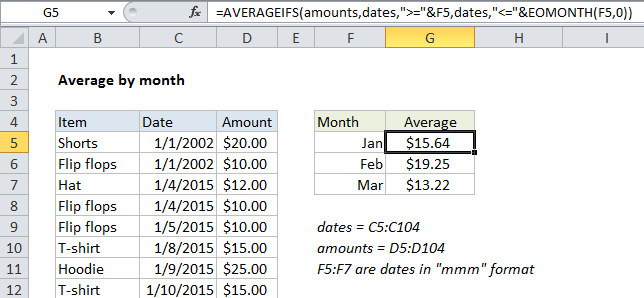
This tutorial shows how to work Average by month in Excel using the example below;

Formula

=AVERAGEIFS(values,dates,">="&A1,dates,"<="&EOMONTH(A1))

Explanation

To average by month, you can use a formula based on the AVERAGEIFS function, with help from the EOMONTH function.

In the example shown, the formula in F4 is:

=AVERAGEIFS(amounts,dates,">="&F5,dates,"<="&EOMONTH(F5,0))

This formula uses the named ranges “amounts” (D5:D104) and “dates” (C5:C104).

How this formula works

The AVERAGEIFS function can average ranges based on multiple criteria. In this case, we configure AVERAGEIFS to average amounts by month using two criteria: (1) match dates greater than or equal to the first day of the month, (2) match dates less than or equal to the last day of the month. If we hard-coded dates for January 2016 into the formula using the DATE function, it would look like this.

=AVERAGEIFS(amounts,dates,">="&DATE(2016,1,1),dates,"<="&DATE(2016,1,31))

But we don’t want to hard-code dates, we want Excel to generate these dates for us. Normally, this is a pain, because if you add month names as text (i.e. “January”, “February”, “March”, etc.) in column E you have to go to extra trouble to create dates you can use for criteria.

However, in this case, we use a simple trick to make things easier: In column E, instead of typing month names, we add actual dates for the first of each month (1/1/2016, 2/1/2016, 3/1/2016, etc.), and use a custom date format (“mmm”) to display the month names.

This makes it easy to build the criteria we need for AVERAGEIFS. To match dates greater than or equal to the first of the month, we use:

">="&E4

And to match dates less than or equal to the last day of the month, we use:

"<="&EOMONTH(E4,0)

EOMONTH automatically returns the last day of the same month because we supply zero for the months argument.

Note: concatenation with an ampersand (&) is necessary when building criteria based on a cell reference.