Map text to numbers in Excel

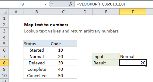
This tutorial shows how to Map text to numbers in Excel using the example below;

Formula

=VLOOKUP(text,lookup_table,2,0)

Explanation

To map or translate text inputs to arbitrary numeric values, you can use the VLOOKUP function with a simple table.

In the example, we need to map five text values (statuses) to numeric status codes as follows:

Since there is no way to derive the output (i.e. it’s arbitrary), we need to do some kind of lookup. The VLOOKUP function provides an easy way to do this.

In the example shown, the formula in F8 is:

=VLOOKUP(F7,B6:C10,2,0)

How this formula works

This formula uses the value in cell F7 for a lookup value, the range B6:C10 for the lookup table, the number 2 to indicate “2nd column”, and zero as the last argument to force an exact match.

Although in this case we are mapping text values to numeric outputs, the same formula can handle text to text, or numbers to text.