How to randomly assign people to groups in Excel

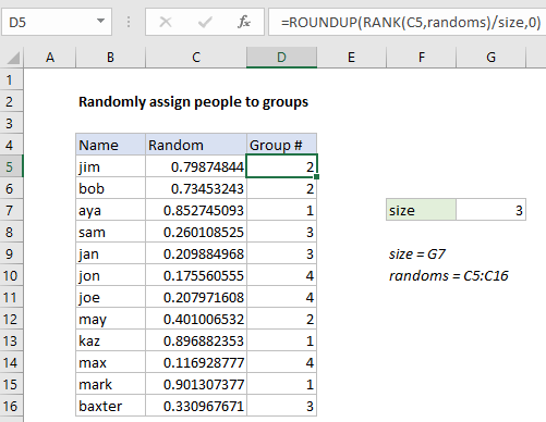
To randomly assign people to groups or teams of a specific size, you can use a helper column with a value generated by the RAND function, together with a formula based on the RANK and ROUNDUP functions.

Formula

=ROUNDUP(RANK(A1,randoms)/size,0)

Explanation

In the example shown, the formula in D5 is:

=ROUNDUP(RANK(C5,randoms)/size,0)

which returns a group number for each name listed in column B, where “randoms” is the named range C5:C16, and “size” is the named range G5.

How this formula works

At the core of this solution is the RAND function, which is used to generate a random number in a helper column (column C in the example).

To assign a full set of random values in one step, select the range C5:C16, and type =RAND() in the formula bar. Then use the shortcut control + enter to enter the formula in all cells at once.

Note: the RAND function will keep generating random values every time a change is made the worksheet, so typically you will want to replace the results in column C with actual values using paste special to prevent changes after random values are assigned.

In column D, a group number is assigned with the following formula:

=ROUNDUP(RANK(C5,randoms)/size,0)

The RANK function is used to rank the value in C5 against all random values in the list. The result will be a number between 1 and the total number of people (12 in this example).

This result is then divided by “size”, which represents the desired group size (3 in the example), which then goes into the ROUNDUP function as number, with num_digits of zero. The ROUNDUP function returns a number rounded up to the next integer. This number represents assigned group number.

CEILING version

The CEILING function can be used instead of ROUNDUP. Like the ROUNDUP function, CEILING also rounds up but instead of rounding to a given number of decimal places, CEILING rounds to a given multiple.

=CEILING(RANK(C5,randoms)/size,1)