Skip to content
Free Excel Tutorials
  • Home
  • Excel For Beginners
  • Excel Intermediate
  • Advanced Excel For Experts

Data Analysis

  • How To Load Analysis ToolPak in Excel
  • Conditional Formatting New Rule with Formulas in Excel
  • How To Insert and Customize Sparklines in Excel
  • Calculate Conditional Percentile ‘IF’ in table in Excel
  • How to Use Solver Tool in Excel

References

  • Create hyperlink with VLOOKUP in Excel
  • How to use Excel COLUMN Function
  • How to use Excel TRANSPOSE Function
  • How to use Excel LOOKUP Function
  • Approximate match with multiple criteria in Excel

Data Validations

  • Excel Data validation no punctuation
  • Excel Data validation don’t exceed total
  • Excel Data validation allow uppercase only
  • Excel Data validation must contain specific text
  • Excel Data validation date in next 30 days

Shade Alternate Rows in Excel

by

This example shows you how to use conditional formatting to shade alternate rows. Shading every other row in a range makes it easier to read your data.
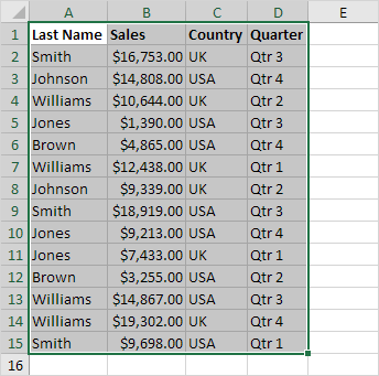
1. Select a range.

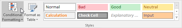
2. On the Home tab, in the Styles group, click Conditional Formatting.

3. Click New Rule.

4. Select ‘Use a formula to determine which cells to format’.

5. Enter the formula =MOD(ROW(),2)

N/B: MOD function under Math & Trig category returns a number after a number is divided by a divisor. Formula tab →Function library group →Math & Trig category  →MOD

6. Select a formatting style and click OK.


Result.

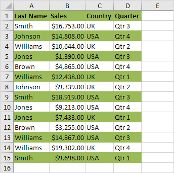
Explanation: the MOD function gives the remainder of a division. The ROW() function returns the row number. For example, for the seventh row, MOD(7,2) equals 1. 7 is divided by 2 (3 times) to give a remainder of 1. For the eight row, MOD(8,2) equals 0. 8 is divided by 2 (exactly 4 times) to give a remainder of 0. As a result, all odd rows return 1 (TRUE) and will be shaded.

Post navigation

Previous Post:

VLOOKUP without #N/A error in Excel

Next Post:

Manipulating text strings using Left, Mid, Right, Len, Substitute in Excel

Leave a Reply Cancel reply

Your email address will not be published. Required fields are marked *

Learn Basic Excel

Ribbon
Workbook
Worksheets
Format Cells
Find & Select
Sort & Filter
Templates
Print
Share
Protect
Keyboard Shortcuts

Categories

  • Charts
  • Data Analysis
  • Data Validation
  • Excel Functions
    • Cube Functions
    • Database Functions
    • Date and Time Functions
    • Engineering Functions
    • Financial Functions
    • Information Functions
    • Logical Functions
    • Lookup and Reference Functions
    • Math and Trig Functions
    • Statistical Functions
    • Text Functions
    • Web Functions
  • Excel VBA
  • Excel Video Tutorials
  • Formatting
  • Grouping
  • Others

Logical Functions

  • Invoice status with nested if in Excel
  • IF with wildcards in Excel
  • IFNA function: Description, Usage, Syntax, Examples and Explanation
  • Complete List of Excel Logical Functions, References and Examples
  • FALSE function: Description, Usage, Syntax, Examples and Explanation

Date Time

  • Get age from birthday in Excel
  • How to get same date next month or previous month in Excel
  • Convert Excel time to decimal seconds
  • How to calculate quarter from date in Excel
  • Add days to date in Excel

Grouping

  • Group numbers at uneven intervals in Excel
  • Group times into unequal buckets in Excel
  • Map inputs to arbitrary values in Excel
  • Group arbitrary text values in Excel
  • How to randomly assign data to groups in Excel

General

  • Excel Ribbon Quick Overview For Beginners
  • Split Cell Content Using Text to Columns in Excel
  • How to generate random number between two numbers in Excel
  • How to create dynamic named range with INDEX in Excel
  • Automatically fill series of cells in Excel using AutoFill
© 2026 xlsoffice . All Right Reserved. | Teal Smiles | Abbreviations And Their Meaning