Highlight unprotected cells in Excel

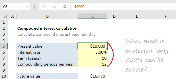
This tutorial shows how to Highlight unprotected cells in Excel using the example below;

Formula

=CELL("PROTECT",A1)=0

Explanation

To highlight unprotected cells (cells that are unlocked) with conditional formatting, you can use a formula based on the CELL function. In the example shown, the custom formula used to set up conditional formatting is:

=CELL("PROTECT",A1)=0

Where A1 represents the active cell in the selection when the rule was defined.

How this formula works

The CELL function can provide a wide range of information about cell properties. One property is called “protect” and indicates whether a cell is unlocked or locked. All cells start out “locked” in a new Excel workbook, but this setting has no effect until a worksheet is protected.

The CELL function returns either 1 or zero to indicate “on” or “off”. In this case we are comparing the result to zero, so when CELL returns 0, the expression returns TRUE and the conditional formatting is triggered. When CELL returns 1, the expression returns FALSE and no conditional formatting is applied.