Highlight duplicate values in Excel

Note: Excel contains many built-in “presets” for highlighting values with conditional formatting, including a preset to highlight duplicate values. However, if you want more flexibility, you can highlight duplicates with your own formula, as explained in this article.

If you want to highlight cells that contain duplicates in a set of data, you can use a simple formula that returns TRUE when a value appears more than once.

For example, if you want to highlight duplicates in the range B4:G11, you can use this formula:

=COUNTIF($B$4:$G$11,B4)>1

Note: with conditional formatting, it’s important that the formula be entered relative to the “active cell” in the selection, which is assumed to be B4 in this case.

How this formula works

COUNTIF simply counts the number of times each value appears in the range. When the count is more than 1, the formula returns TRUE and triggers the rule.

When you use a formula to apply conditional formatting, the formula is evaluated relative to the active cell in the selection at the time the rule is created. In this case, the range we are using in COUNTIF is locked with an absolute address, but B4 is fully relative. So, the rule is evaluated for each cell in the range, with B4 changing and $B$4:$G$11 remaining unchanged.

A variable number of duplicates + named ranges

Instead of hard-coding the number 1 into the formula you can reference a cell to make the number of duplicates variable.

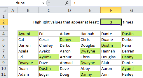
You can extend this idea and make the formula easier to read by using named ranges. For example, if you name G2 “dups”, and the range B4:G11 “data”, you can rewrite the formula like so:

=COUNTIF(data,B4)>=dups

You can then change the value in G2 to anything you like and the conditional formatting rule will respond instantly, highlighting cell that contain values greater than or equal to the number you put in the named range “dups”.