Highlight dates in same month and year in Excel
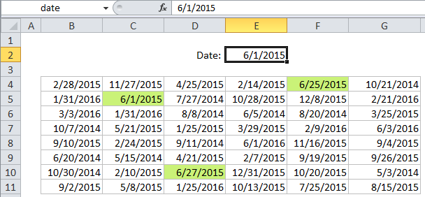
This tutorial shows how to Highlight dates in same month and year in Excel using the example below;
Formula
=TEXT(A1,"myyyy")=TEXT(date,"myyyy")

Explanation
If you want to use conditional formatting to highlight dates that are in the same month and year as another date, you can use a simple formula based on the TEXT function.
For example, if you have dates in the range B4:G11, and want to highlight dates that have the same month and year as the date June 1, 2015, select the range B4:G11 and create a new CF rule that uses this formula:
=TEXT(B4,"myyyy")=TEXT(DATE(2015,6,1),"myyyy")
Note: it’s important that CF formulas be entered relative to the “active cell” in the selection, which is assumed to be B4 in this case.
Once you save the rule, you’ll see all dates that occur in June 2015 highlighted.
How this formula works
This formula uses the TEXT function to concatenate the month and year of each date. Then, the two dates are tested for equality. TEXT is a useful function that allows you to convert a number to text in the text format of your choice. In this case the format is the custom date format “myyyy”, which translates to: month number without leading zeros & 4-digit year. For example, if A1 contains the date 9-Jun-2015, TEXT(A1,”myyyy”) will produce the text string “62016”.
Use other cells for input
You don’t need to hard-code a date into the rule. To make a more flexible rule, you can use another cells like a variable. For example, if you name cell E2 “date”, you can rewrite the formula like so:
=TEXT(B4,"myyyy")=TEXT(date,"myyyy")
Then whenever you change the date in E2, the conditional formatting rule will update instantly. This simplifies the formula and makes it easier to read.