Highlight dates between in Excel

=AND(A1>=date1,A1<=date2)

Explanation

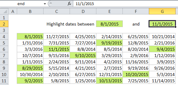
If you want to highlight dates between two dates with conditional formatting, you can use a simple formula that uses the AND and DATE functions together. For example, if you have dates in the range B4:G11, and want to highlight cells that contain a date greater than August 1st, 2015, and less than November 1, 2015, select the range and create a new CF rule that uses this formula:

=AND(B4>=DATE(2015,8,1),B4<=DATE(2015,11,1))

Note: it’s important that CF formulas be entered relative to the “active cell” in the selection, which is assumed to be B4 in this case.

Once you save the rule, you’ll see the dates between 8/1/2015 and 11/1/2015 are highlighted. Note we are including the start and end dates by using greater than or equal to (>=) and less than or equal to (<=)

How this formula works

The AND function takes multiple arguments and returns TRUE only when all arguments return TRUE. The DATE function creates a proper Excel date with given year, month, and day values. Because the reference to B4 is fully relative, it will update as the rule is applied to each cell in the range, and any dates that are both greater than 8/1/2015 and less than 11/1/2015 will be highlighted.

Use other cells for input

You don’t need to hard-code the dates into the rule. To make a more flexible rule, you can use other cells like variables in the formula. For example, you can name cell E2 “start” and cell G2 “end”, then rewrite the formula like so:

=AND(B4>=start,B4<=end)

When you change either date, the conditional formatting rule will respond instantly. By using other cells for input, and naming them as named ranges, you make the conditional formatting interactive and the formula is simpler and easier to read.