Highlight blank cells in Excel

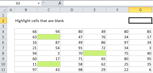
This tutorial shows how to Highlight blank cells in Excel using the example below;

Formula

=ISBLANK(A1)

Explanation

If you want to highlight cells that are blank or empty with conditional formatting, you can do so with a simple formula based on the ISBLANK function. For example, if you want to highlight blank cells in the range B4:G11, just select the range and create a conditional formatting rule based on this formula:

=ISBLANK(B4)

Note: it’s important that CF formulas be entered relative to the “active cell” in the selection, which is assumed to be B4 in this case.

Once you save the rule, you’ll see the formatting applied to all empty cells.

How this formula works

When you use a formula to apply conditional formatting, the formula is evaluated relative to the active cell in the selection at the time the rule is created. So, in this case the formula =ISBLANK(B4) is evaluated for each cells in B4:G11. Because B4 is entered as a relative address, the address will be updated each time the formula is applied, and ISBLANK() is run on each cell in the range.

Empty vs. blank

The ISBLANK function only returns true when cell are actually empty. If a cell contains a formula that returns an empty string (i.e. “”) ISBLANK won’t see these cells as blank, and won’t return true, so they won’t be highlighted. In this way, ISBLANK would be better thought of as “ISEMPTY” (Hat tip, Mike Girvin).

If you want to highlight all cells that are blank and cells that just appear blank, you can use this formula instead:

=LEN(B4)=0

The LEN formula returns the length of text as a number. The formula LEN(B4)=0, will return true for both “blank” and “empty” cells.