Highlight 3 smallest values with criteria in Excel

This tutorial shows how to Highlight 3 smallest values with criteria in Excel using the example below;

Formula

=AND(A1=criteria,B1<=SMALL(IF(criteria,values),3))

Explanation

To highlight the 3 smallest values that meet specific criteria, you can use an array formula based on the AND and SMALL functions.

In the example shown, the formula used for conditional formatting is:

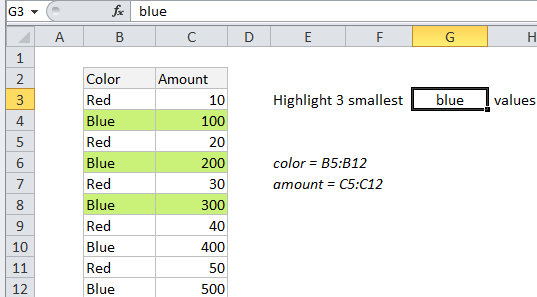
=AND($B3=$G$3,$C3<=SMALL(IF(color=$G$3,amount),3))

Where “color” is the named range B5:B12 and “amount” is the named range C5:C12.

How this formula works

Inside the AND function there are two logical criteria. The first is straightforward, and ensures that only cells that match the color in G3 are highlighted:

$B3=$G$3

The second logical is more complex. It’s an array formula that filters all amounts to make sure that only amounts associated with the color in G3 are highlighted:

$C3<=SMALL(IF(color=$G$3,amount),3)

The filtering is done with the IF function here:

IF(color=$G$3,amount)

The value from the amount column only survives if the color in column B matches the value in G3. The resulting array looks like this:

{FALSE;100;FALSE;200;FALSE;300;FALSE;400;FALSE;500}

and goes into the SMALL function with a k value of 3.

SMALL returns the “3rd smallest” value and only values less than or equal to this value return true.

When both logical conditions are return TRUE, the conditional formatting is triggered and cells are highlighted.

Note: this is an array formula, but it doesn’t require control + shift + enter like an array formula entered directly on a worksheet.