Conditional formatting date past due in Excel

This tutorial shows how to work Conditional formatting date past due in Excel using the example below;

Formula

=A1<TODAY()

Explanation

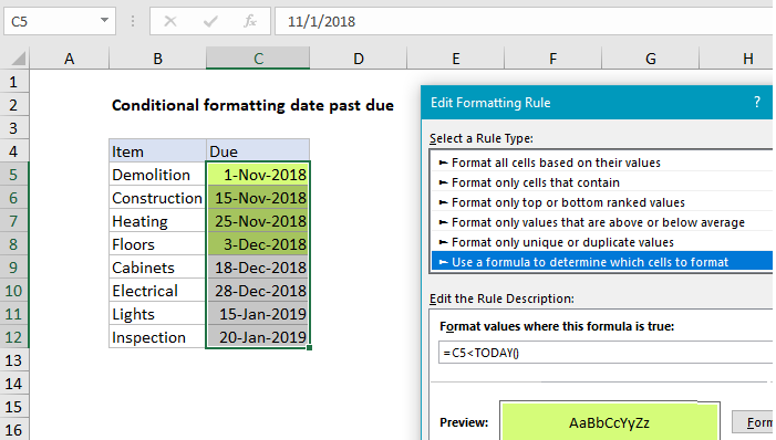
To highlight dates that are “past due” you can use a conditional formatting and a basic formula to check whether each date is less than today. In the example shown, conditional formatting has been applied to the range C5:C12 with this formula:

=C5<TODAY()

When a date in column C is less than the date TODAY (i.e. past due), the formula returns TRUE and triggers the rule.

Note: conditional formatting formulas should be entered relative to the “active cell” in the selection, which is assumed to be C5 in this case.

How this formula works

When conditional formatting is applied with a formula, the formula is evaluated relative to the active cell in the selection at the time the rule is created. In this case, the active cell when the rule is created is assumed to be cell C5, with the range C5:C12 selected.

As the formula is evaluated, formula references change so that the rule is testing for blank values in the correct row for each of the 8 cells in the range:

=C5<TODAY() // C5
=C6<TODAY() // C6
=C7<TODAY() // C7
etc.

Since Excel dates are by just serial numbers, any past due date is, by definition, less than the current date, which isgenerated with the TODAY function. This article was created December 17, 2018, so all earlier dates return TRUE and are highlighed by the rule. Dates greater than or equal today return FALSE so no shading is applied.

Overdue by at least n days

To test if dates are overdue by at least N days, you can use this formula:

=(TODAY()-C5)>=N

This formula will trigger conditional formatting only when a date in column C is at least n days earlier than today.