Clean and reformat telephone numbers using SUBSTITUTE function in Excel
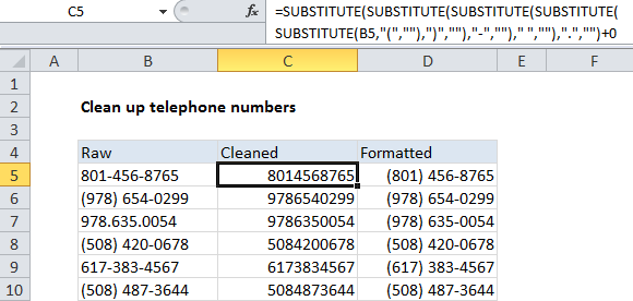
One way to clean up and reformat telephone numbers is to strip out all extraneous characters, then apply Excel’s built-in telephone number format.
Formula
=SUBSTITUTE(SUBSTITUTE(SUBSTITUTE
(SUBSTITUTE(SUBSTITUTE(A1,"(",""),
")",""),"-","")," ",""),".","")+0

Note that the cell appears in the middle, with function names above and substitutions below. Not only does this make the formula easier to read, it also makes it easier to add and remove
Explanation
This formula above uses a series of nested SUBSTITUTE functions to strip out spaces, hyphens, periods, parentheses, and commas.
You’ll need to adjust the actual replacements to suit your data.
How this formula works
The formula runs from the inside out, with each SUBSTITUTE removing one character.
The inner most SUBSTITUTE removes the left parentheses, and the result is handed to the next SUBSTITUTE, which removes the right parentheses, and so on.
Whenever you use the SUBSTITUTE function, the result will be text. Because you can’t apply a number format to text, we need to convert the text to a number. One way to do that is to add zero (+0), which automatically converts numbers in text format to numbers in numeric format.
Finally, the “Special” telephone number format is applied (column D).
This page explains custom number formats and with many examples.
White space trick for better readability
When nesting multiple functions, it can be difficult to read the formula and keep all parentheses balanced. Excel doesn’t care about extra white space in a formula, so you can add line breaks in the formula to make the formula more readable. For example, the formula above can be written as follows:
=
SUBSTITUTE(
SUBSTITUTE(
SUBSTITUTE(
SUBSTITUTE(
SUBSTITUTE(
A1,
"(",""),
")",""),
"-",""),
" ",""),
".","")