How to strip non-numeric characters in Excel

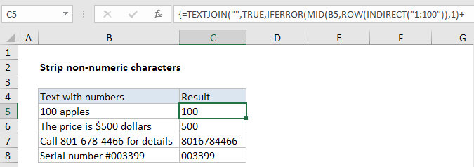
To remove non-numeric characters from a text string, you can try this experimental formula based on the TEXTJOIN function, new in Excel 2016.

Formula

{=TEXTJOIN("",TRUE,IFERROR(MID(A1,ROW
(INDIRECT("1:100")),1)+0,""))}

Note: TEXTJOIN will return the numbers as text, for example “100,”500″, etc. If you want a true numeric result, add zero, or wrap the entire formula in the VALUE function. TEXTJOIN was added in Excel 2016 + Office 365.

Explanation

In the example shown, the formula in C5 is:

{=TEXTJOIN("",TRUE,IFERROR(MID(B5,ROW
(INDIRECT("1:100")),1)+0,""))}

Note: this is an array formula and must be entered with control + shift + enter.

How this formula works

Working from the inside out, the MID formula is used to extract the text in B5, one character at a time.  The key is the ROW/INDIRECT piece:

ROW(INDIRECT("1:100"))

which spins up an array containing 100 numbers like this:

{1,2,3,4,5,6,7,8….99,100}

Note: 100 represents the maximum characters to process. Change to suit your data.

This array goes into the MID function as the start_num argument. For num_chars, we use 1.

The MID function returns an array like this:

{“1″;”0″;”0″;” “;”a”;”p”;”p”;”l”;”e”;”s”;””;””;””;””…}

(extra items in the array removed for readability)

To this array, we add zero. This is a simple trick that forces Excel to try and coerce text to a number. Numeric text values like “1”,”2″,”3″,”4″ etc. are converted, while non-numeric values fail and throw a #VALUE error. We use the IFERROR function to catch these errors and return an empty string, while numeric values pass through into the array. The result is an array that contains just numbers and empty strings:

{1;0;0;””;””;””;””;””;….}

Finally, this array result goes into the TEXTJOIN function as the text1 argument. For delimiter, we use an empty string (“”) and for ignore_empty we supply TRUE. TEXTJOIN then concatenates all non-empty values in the array and returns the result.