Skip to content
Free Excel Tutorials
  • Home
  • Excel For Beginners
  • Excel Intermediate
  • Advanced Excel For Experts

Data Analysis

  • Working With Tables in Excel
  • Excel Frequency Function Example
  • Conditional Formatting Color Scales Examples in Excel
  • Move chart to a separate worksheet in Excel
  • How to do a t-Test in Excel?

References

  • INDEX function: Description, Usage, Syntax, Examples and Explanation
  • Merge tables with VLOOKUP in Excel
  • How to get address of named range in Excel
  • How to reference named range different sheet in Excel
  • Extract all partial matches in Excel

Data Validations

  • Excel Data validation allow uppercase only
  • Excel Data validation don’t exceed total
  • Excel Data validation must begin with
  • Excel Data validation whole percentage only
  • Excel Data validation number multiple 100

How to get last line in cell in Excel

by

To get the last word from a text string, you can use a formula based on the TRIM, SUBSTITUTE, RIGHT, and REPT functions.

Formula

=TRIM(RIGHT(SUBSTITUTE(B5,CHAR(10),REPT(" ",200)),200))

Note: 200 is an arbitrary number that represents the longest line you expect to find in a cell. If you have longer lines, increase this number as needed.

Explanation

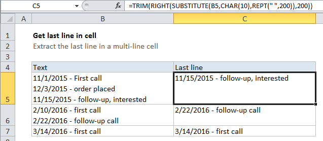
In the example shown, the formula in C5 is:

=TRIM(RIGHT(SUBSTITUTE(B5,CHAR(10),REPT(" ",200)),200))

How this formula works

This formula takes advantage of the fact that TRIM will remove any number of leading spaces. We look for line breaks and “flood” the text with spaces where we find one. Then we come back and grab text from the right.

Working from the inside out, we use the SUBSTITUTE function to find all line breaks (char 10)  in the text, and replace each one with 200 spaces:

SUBSTITUTE(B5,CHAR(10),REPT(" ",200))

After the substitution, the looks like this (with hyphens marking spaces for readability):

line one----------line two----------line three

With 200 spaces between each line of text.

Next, the RIGHT function extracts 200 characters, starting from the right. The result will look like this:

-------line three

Finally, the TRIM function removes all leading spaces, and returns the last line.


Post navigation

Next Post:

Create One-dimensional and Two-dimensional Array

Leave a Reply Cancel reply

Your email address will not be published. Required fields are marked *

Learn Basic Excel

Ribbon
Workbook
Worksheets
Format Cells
Find & Select
Sort & Filter
Templates
Print
Share
Protect
Keyboard Shortcuts

Categories

  • Charts
  • Data Analysis
  • Data Validation
  • Excel Functions
    • Cube Functions
    • Database Functions
    • Date and Time Functions
    • Engineering Functions
    • Financial Functions
    • Information Functions
    • Logical Functions
    • Lookup and Reference Functions
    • Math and Trig Functions
    • Statistical Functions
    • Text Functions
    • Web Functions
  • Excel VBA
  • Excel Video Tutorials
  • Formatting
  • Grouping
  • Others

Logical Functions

  • Return blank if in Excel
  • How to use Excel FALSE Function
  • NOT function: Description, Usage, Syntax, Examples and Explanation
  • IFERROR function: Description, Usage, Syntax, Examples and Explanation
  • Nested IF function example in Excel

Date Time

  • Convert Unix time stamp to Excel date
  • Series of dates by day
  • Convert decimal seconds to Excel time
  • Calculate days remaining in Excel
  • How to calculate working days left in month in Excel

Grouping

  • Group numbers at uneven intervals in Excel
  • If cell contains one of many things in Excel
  • Map text to numbers in Excel
  • Calculate conditional mode with criteria in Excel
  • Group numbers with VLOOKUP in Excel

General

  • Basic error trapping example in Excel
  • How to get original price from percentage discount in Excel
  • Count cells that contain errors in Excel
  • How to Create Calendar in Excel
  • Subtotal invoices by age in Excel
© 2026 xlsoffice . All Right Reserved. | Teal Smiles | Abbreviations And Their Meaning