How to display conditional message with REPT function in Excel

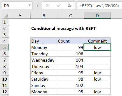
 In the example shown, the formula in D5 (copied down) is:

=REPT("low",C5<100)

If the value in column C is less than 100, the formula returns “low”. If not, the formula returns an empty string (“”), which looks like a blank cell.

How this formula works

This formula uses boolean logic to output a conditional message. If the value in column C is less than 100, the formula returns “low”. If not, the formula returns an empty string (“”).

Boolean logic is a technique of handling TRUE and FALSE values like 1 and 0. In cell C5, the formula is evaluated like this:

=REPT("low",C5<100)
=REPT("low",TRUE)
=REPT("low",1)
="low"

In other words, if C5 < 100, output “low” 1 time. In cell C6, the formula is evaluated like this:

=REPT("low",C6<100)
=REPT("low",FALSE)
=REPT("low",0)
=""

In other words, if C6 < 100 is FALSE, output “low” zero times.

IF function alternative

Conditional messages like this are more commonly handled with the IF function. With IF, the equivalent formula is:

=IF(C5<100,"low","")

Both formulas return exactly the same result, but the REPT version is a bit simpler.

Extending the logic

Boolean logic can be extended with simple math operations to handle more complex scenarios. Briefly, AND logic can be expressed with multiplication (*)  OR logic can be expressed with addition (+).  For example, to return “low” only when (count < 100) AND  (day = Monday) we can use boolean logic like this:

=REPT("low",(C5<100)*(B5="Monday"))

The equivalent IF formula is:

=IF(C5<100,IF(B5="Monday","low",""),"")

or, simplifying a bit with AND:

=IF(AND(C5<100,B5="Monday"),"low","")

Coercing TRUE and FALSE to 1 and zero

When using boolean logic, you’ll sometimes need to force Excel to coerce TRUE and FALSE to 1 and zero. A simple way to do this is to use a double-negative (–).