Extract most frequently occurring text in Excel

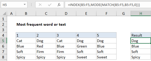
In the example shown, the formula in H5 is:

=INDEX(B5:F5,MODE(MATCH(B5:F5,B5:F5,0)))

Working from the inside out, the MATCH function matches the range against itself. That is, we give the MATCH function the same range for lookup value and lookup array (B5:F5).

Because the lookup value contains more than one value (an array), MATCH returns an array of results, where each number represents a position. In the example shown, the array looks like this:

{1,2,1,2,2}

Wherever “dog” appears, we see 2, and Wherever “cat” appears, we see 1. That’s because the MATCH function always returns the first match, which means subsequent occurrences of a given value will return the same (first) position.

Next, this array is fed into the MODE function. MODE returns the most frequently occurring number, which in this case is 2. The number 2 represents the position at which we’ll find the most frequently occurring value in the range.

Finally, we need to extract the value itself. For this, we use the INDEX function. For array, we use the range of values (B5:F5). The row number is provided by MODE.

INDEX returns the value at position 2, which is “dog”.

Empty cells

To deal with empty cells, you can use the following array formula, which adds an IF statement to test for empty cells:

{=INDEX(B5:F5,MODE(IF(B5:F5<>"",MATCH(B5:F5,B5:F5,0))))}

This is an array formula, and must be entered with control + shift + enter.