Sum last n columns in Excel
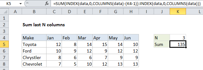
This tutorial shows how to Sum last n columns in Excel using the example below;
Formula
=SUM(INDEX(data,0,COLUMNS(data)-(n-1)):INDEX(data,0,COLUMNS(data)))

Explanation
To sum the last n columns in a table of data (i.e. last 3 columns, last 4 columns, etc.) you can use a formula based on the INDEX function. In the example shown, the formula in K5:
=SUM(INDEX(data,0,COLUMNS(data)-(K4-1)):
INDEX(data,0,COLUMNS(data)))
where “data” is the named range C5:H8
How this formula works
The key to understanding this formula is to realize that the INDEX function can be used to return a reference to entire rows and entire columns.
To generate a reference to the “last n columns” in a table, we build a reference in two parts, joined by the range operator. To get a reference to the left column, we use:
INDEX(data,0,COLUMNS(data)-(K4-1))
Since data contains 6 columns, and K4 contains 3, this simplifies to:
INDEX(data,0,4) // all of column 4
To get a reference to the right column in the range, we use:
INDEX(data,0,COLUMNS(data))
Which returns a reference to column 6 of the named range “data”, since the COLUMN function returns 6:
INDEX(data,0,6) // all of column 6
Together, the two INDEX functions return a reference to columns 4 through 6 in the data (i.e. F5:H8), which resolve to an array of values inside the SUM function:
SUM({15,14,10;9,12,12;7,9,9;12,13,13})
The SUM function then calculates and returns the sum, 135.