Excel Get integer part of a number Example

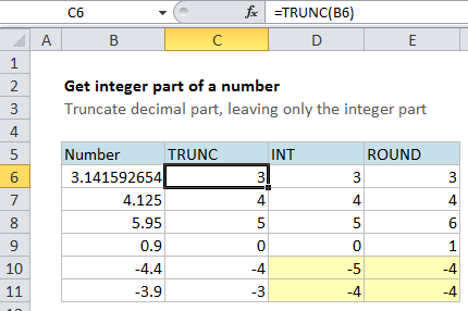
In the example, cell C6 contains this formula:

=TRUNC(B6)

The TRUNC function simply truncates (i.e. removes) numbers; it doesn’t not round at all.

How this formula works

With TRUNC, no rounding takes place. The TRUNC function simply slices off the decimal part of the number with default settings.

TRUNC actually takes an optional second argument to specify the precision of truncation, but when you don’t supply this optional argument, it is assumed to be zero, and truncation happens at the decimal.

What about INT or ROUND?

You might wonder if you can use the INT or ROUND functions instead.

The behavior of INT is identical to TRUNC (with default settings) for positive numbers — the INT function will round a number down to the next integer and then return only the integer portion of the number.

However, for negative numbers, the rounding that INT does is a bit strange.

This is because INT rounds negative numbers down away from zero, no matter what the decimal value. See the last 2 examples in the screen above for an example.

Because of this behavior, TRUNC is a better option if you just want the integer portion of a number.

As you would expect, the ROUND function rounds numbers down. If you want to round to the nearest integer, (positive or negative) just use:

=ROUND(number,0)

But be aware that the integer value may be different than the number you started with due to rounding.