LOOKUP function: Description, Usage, Syntax, Examples and Explanation
What is Excel LOOKUP function ?
LOOKUP function is one of the lookup and reference functions in Microsoft office Excel that is used to return a value from a range (one row or one column) or from an array. When you need to look in a single row or column and find a value from the same position in a second row or column, use LOOKUP function.
There are 2 different syntaxes for the LOOKUP function:
LOOKUP Function (Syntax #1)
In Syntax #1, the LOOKUP function searches for value in the lookup_range and returns the value in the result_rangethat is in the same position.
The syntax for the LOOKUP function in Microsoft Excel is:
LOOKUP( value, lookup_range, [result_range] )
LOOKUP formula explanation
- value
- The value to search for in the lookup_range.
- lookup_range
- A single row or single column of data that is sorted in ascending order. The LOOKUP function searches for value in this range.
- result_range
- Optional. It is a single row or single column of data that is the same size as the lookup_range. The LOOKUP function searches for the value in the lookup_range and returns the value from the same position in the result_range. If this parameter is omitted, it will return the first column of data.
Returns
The LOOKUP function returns any datatype such as a string, numeric, date, etc.
If the LOOKUP function can not find an exact match, it chooses the largest value in the lookup_range that is less than or equal to the value.
If the value is smaller than all of the values in the lookup_range, then the LOOKUP function will return #N/A.
If the values in the LOOKUP_range are not sorted in ascending order, the LOOKUP function will return the incorrect value.
Example of LOOKUP function
Example 1

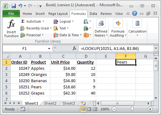
Based on the Excel spreadsheet above, the following LOOKUP examples would return:
=LOOKUP(10251, A1:A6, B1:B6)
Result: "Pears"

=LOOKUP(10251, A1:A6)
Result: 10251

=LOOKUP(10246, A1:A6, B1:B6)
Result: #N/A

=LOOKUP(10248, A1:A6, B1:B6)
Result: "Apples"
LOOKUP Function (Syntax #2)
In Syntax #2, the LOOKUP function searches for the value in the first row or column of the array and returns the corresponding value in the last row or column of the array.
The syntax for the LOOKUP function in Microsoft Excel is:
LOOKUP( value, array )
Parameters or Arguments
- value
- The value to search for in the array. The values must be in ascending order.
- array
- An array of values that contains both the values to search for and return.
Returns
The LOOKUP function returns any datatype such as a string, numeric, date, etc.
If the LOOKUP function can not find an exact match, it chooses the largest value in the lookup_range that is less than or equal to the value.
If the value is smaller than all of the values in the lookup_range, then the LOOKUP function will return #N/A.
If the values in the array are not sorted in ascending order, the LOOKUP function will return the incorrect value.
Example 2
Let’s look at some Excel LOOKUP function examples and explore how to use the LOOKUP function as a worksheet function in Microsoft Excel:
=LOOKUP("T", {"s","t","u","v";10,11,12,13})
Result: 11

=LOOKUP("Tech on the Net", {"s","t","u","v";10,11,12,13})
Result: 11

=LOOKUP("t", {"s","t","u","v";"a","b","c","d"})
Result: "b"

=LOOKUP("r", {"s","t","u","v";"a","b","c","d"})
Result: #N/A

=LOOKUP(2, {1,2,3,4;511,512,513,514})
Result: 512