How to use Excel VLOOKUP Function

Excel VLOOKUP Function Description

VLOOKUP is an Excel function to lookup and retrieve data from a specific column in table. The VLOOKUP function performs a vertical lookup by searching for a value in the first column of a table and returning the value in the same row in the index_number position.

VLOOKUP supports approximate and exact matching, and wildcards (* ?) for partial matches. The “V” stands for “vertical”. Lookup values must appear in the first column of the table, with lookup columns to the right.

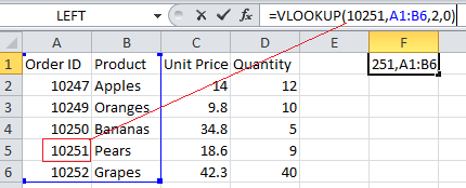
Explanation: Based on example  above, the VLOOKUP function would return:

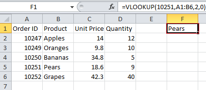
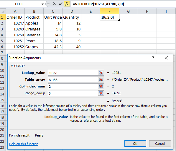
=VLOOKUP(10251, A1:B6, 2, FALSE)
Result: "Pears"   'Returns value in 2nd column

=VLOOKUP(10248, A1:B6, 2, FALSE)
Result: #N/A      'Returns #N/A error (no exact match)

=VLOOKUP(10248, A1:B6, 2, TRUE)
Result: "Apples"  'Returns an approximate match

VLOOKUP( value, table, index_number, [approximate_match] )

Exact Match vs. Approximate Match

To find an exact match, use FALSE as the final parameter. To find an approximate match, use TRUE as the final parameter.

Let’s lookup a value that does not exist in our data to demonstrate the importance of this parameter!

Exact Match

Use FALSE to find an exact match:

=VLOOKUP(10248, A1:B6, 2, FALSE)
Result: #N/A

If no exact match is found, #N/A is returned.

Approximate Match

Use TRUE to find an approximate match:

=VLOOKUP(10248, A1:B6, 2, TRUE)
Result: "Apples"

If no match is found, it returns the next smaller value which in this case is “Apples”.

VLOOKUP from Another Sheet

You can use the VLOOKUP to lookup a value when the table is on another sheet. Let’s modify our example above and assume that the table is in a different Sheet called Sheet2 in the range A1:B6.

We could rewrite our original example where we lookup the value 10251 as follows:

=VLOOKUP(10251, Sheet2!A1:B6, 2, FALSE)

By preceding the table range with the sheet name and an exclamation mark, we can update our VLOOKUP to reference a table on another sheet.

VLOOKUP from Another Sheet with Spaces in Sheet Name

Let’s throw in one more complication. What happens if your sheet name contains spaces? If there are spaces in the sheet name, you will need to change the formula further.

Let’s assume that the table is on a Sheet called “Test Sheet” in the range A1:B6, now we need to wrap the Sheet name in single quotes as follows:

=VLOOKUP(10251, 'Test Sheet'!A1:B6, 2, FALSE)

By placing the sheet name within single quotes, we can handle a sheet name with spaces in the VLOOKUP function.

VLOOKUP from Another Workbook

You can use the VLOOKUP to lookup a value in another workbook. For example, if you wanted to have the table portion of the VLOOKUP formula be from an external workbook, we could try the following formula:

=VLOOKUP(10251, 'C:\[data.xlsx]Sheet1'!$A$1:$B$6, 2, FALSE)

This would look for the value 10251 in the file C:\data.xlxs in Sheet 1 where the table data is found in the range $A$1:$B$6.

Why use Absolute Referencing?

Now it is important for us to cover one more mistake that is commonly made. When people use the VLOOKUP function, they commonly use relative referencing for the table range like we did in some of our examples above. This will return the right answer, but what happens when you copy the formula to another cell? The table range will be adjusted by Excel and change relative to where you paste the new formula. Let’s explain further…

So if you had the following formula in cell G1:

=VLOOKUP(10251, A1:B6, 2, FALSE)

And then you copied this formula from cell G1 to cell H2, it would modify the VLOOKUP formula to this:

=VLOOKUP(10251, B2:C7, 2, FALSE)

Since your table is found in the range A1:B6 and not B2:C7, your formula would return erroneous results in cell H2. To ensure that your range is not changed, try referencing your table range using absolute referencing as follows:

=VLOOKUP(10251, $A$1:$B$6, 2, FALSE)

Now if you copy this formula to another cell, your table range will remain $A$1:$B$6.

How to Handle #N/A Errors

Next, let’s look at how to handle instances where the VLOOKUP function does not find a match and returns the #N/A error. In most cases, you don’t want to see #N/A but would rather display a more user-friendly result.

For example, if you had the following formula:

=VLOOKUP(10248, $A$1:$B$6, 2, FALSE)

Instead of displaying #N/A error if you do not find a match, you could return the value “Not Found”. To do this, you could modify your VLOOKUP formula as follows:

=IF(ISNA(VLOOKUP(10248, $A$1:$B$6, 2, FALSE)), "Not Found", VLOOKUP(10248, $A$1:$B$6, 2, FALSE))

OR

=IFERROR(VLOOKUP(10248, $A$1:$B$6, 2, FALSE), "Not Found")

OR

=IFNA(VLOOKUP(10248, $A$1:$B$6, 2, FALSE), "Not Found")

These formulas use the ISNA, IFERROR and IFNA functions to return “Not Found” if a match is not found by the VLOOKUP function.

This is a great way to spruce up your spreadsheet so that you don’t see traditional Excel errors.