Skip to content
Free Excel Tutorials
  • Home
  • Excel For Beginners
  • Excel Intermediate
  • Advanced Excel For Experts

Data Analysis

  • Excel Pie Chart
  • How to Sort by Color in Excel
  • Calculate Conditional Percentile ‘IF’ in table in Excel
  • Conflicting Multiple Conditional Formatting Rules in Excel
  • How to calculate average last N values in a table in Excel

References

  • Perform case-sensitive Lookup in Excel
  • How to get relative row numbers in a range in Excel
  • How to get last row in text data in Excel
  • Find closest match in Excel
  • How to get first row number in range in Excel

Data Validations

  • Excel Data validation date in next 30 days
  • Excel Data validation must begin with
  • Excel Data validation allow weekday only
  • Excel Data validation exists in list
  • Prevent invalid data entering in specific cells

How to use Excel INDIRECT Function

by

This Excel tutorial explains how to use the INDIRECT function with syntax and examples.

Excel INDIRECT function Description

Microsoft Excel INDIRECT function returns the reference to a cell based on its string representation.

The INDIRECT function is a built-in function in Excel that is categorized as a Lookup/Reference Function that can be entered as part of a formula in a cell of a worksheet.

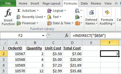
Explanation: Based on the example above, the INDIRECT function would return:

=INDIRECT("$B$4")
Result: 3

=INDIRECT("A5")
Result: 10570

=INDIRECT("A5", TRUE)
Result: 10570

=INDIRECT("R2C3", FALSE)
Result: $3.50

Syntax

The syntax for the INDIRECT function in Microsoft Excel is:

INDIRECT( string_reference, [ref_style] )

Arguments

string_reference
A textual representation of a cell reference.
ref_style
Optional. It is either a TRUE or FALSE value. TRUE indicates that string_reference will be interpreted as an A1-style reference. FALSE indicates that string_reference will be interpreted as an R1C1-style reference. If this parameter is omitted, it will interpret string_reference as an A1-style.

Returns

The INDIRECT function returns the reference to a cell and thus displays the referenced cell’s value.

Post navigation

Previous Post:

VLOOKUP without #N/A error in Excel

Next Post:

Manipulating text strings using Left, Mid, Right, Len, Substitute in Excel

Leave a Reply Cancel reply

Your email address will not be published. Required fields are marked *

Learn Basic Excel

Ribbon
Workbook
Worksheets
Format Cells
Find & Select
Sort & Filter
Templates
Print
Share
Protect
Keyboard Shortcuts

Categories

  • Charts
  • Data Analysis
  • Data Validation
  • Excel Functions
    • Cube Functions
    • Database Functions
    • Date and Time Functions
    • Engineering Functions
    • Financial Functions
    • Information Functions
    • Logical Functions
    • Lookup and Reference Functions
    • Math and Trig Functions
    • Statistical Functions
    • Text Functions
    • Web Functions
  • Excel VBA
  • Excel Video Tutorials
  • Formatting
  • Grouping
  • Others

Logical Functions

  • Invoice status with nested if in Excel
  • How to use IFS function in Excel
  • Check multiple cells are equal in Excel
  • How to use Excel TRUE Function
  • OR function Examples in Excel

Date Time

  • Convert text date dd/mm/yy to mm/dd/yy in Excel
  • Get days, hours, and minutes between dates in Excel
  • Convert date string to date time in Excel
  • How to calculate percent of year complete in Excel
  • Display the current date in Excel

Grouping

  • How to randomly assign data to groups in Excel
  • Map inputs to arbitrary values in Excel
  • Map text to numbers in Excel
  • Group numbers at uneven intervals in Excel
  • Categorize text with keywords in Excel

General

  • How to make excel worksheets print on one page?
  • Delete Blank Rows at Once in Excel
  • Zoom Worksheet in Excel
  • Index and match on multiple columns in Excel
  • How to Create Calendar in Excel
© 2026 xlsoffice . All Right Reserved. | Teal Smiles | Abbreviations And Their Meaning